Algebraic & Mathematical Blocks

Blocks that compute an output directly from their inputs, with no internal dynamics.

---

abs

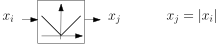
Absolute value of input.

Syntax

& abs
x_i
x_j

x_i is the input state; x_j is the output state (the absolute value of x_i).

Internal states: none

Discrete variable: $z \in \{-1, 1\}$

Equations

$$0 = \begin{cases} x_j - x_i & \text{if } z = 1 \\ x_j + x_i & \text{if } z = -1 \end{cases}$$

Discrete transitions

if z = 1:
    if x_i < 0:
        z ← -1
else:  # z = -1
    if x_i > 0:
        z ← 1

Initialization

if x_i > 0:
    z ← 1
else:
    z ← 0

Notes

The model has a discontinuous derivative at $x_i = 0$. It is implemented internally with a small hysteresis; see the hyst block with $x_I = \epsilon$, $y_{IB} = -\epsilon$, $y_{IA} = \epsilon$, $x_D = -\epsilon$, $y_{DB} = -\epsilon$, $y_{DA} = \epsilon$, where $\epsilon$ is the absolute accuracy used to solve the algebraic equations in RAMSES.

---

algeq

Algebraic equation.

Syntax

& algeq
math expression

Internal states: none

Discrete variables: none

Description

This block forces an algebraic constraint (or equation) involving one or several states:

$f(x_1, x_2, \ldots, x_n) = 0$

where $n$ is the number of states ($n \ge 1$).

Notes

This block does not have distinct “inputs” and “outputs”. Those roles emerge from the rest of the model that incorporates the algebraic constraint.

---

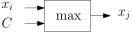
max1v1c

Maximum between a state and a constant.

Syntax

& max1v1c
x_i
x_j
{C}

x_i is the input state, x_j is the output ($\max(x_i, C)$), and C is a constant (data name, parameter name, or math expression).

Internal states: none

Discrete variable: $z \in \{1, 2\}$

Equations

$$0 = \begin{cases} x_j - C & \text{if } z = 1 \\ x_j - x_i & \text{if } z = 2 \end{cases}$$

When $z = 1$ the output is clamped to $C$; when $z = 2$ the output tracks $x_i$.

Discrete transitions

if z = 1:
    if x_i > C:
        z ← 2
else:  # z = 2
    if x_i <= C:
        z ← 1

Initialization

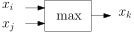
if x_i < C:
    z ← 1
else:
    z ← 2

---

max2v

Maximum between two states.

Syntax

& max2v
x_i
x_j
x_k

x_i and x_j are the two input states; x_k is the output ($\max(x_i, x_j)$).

Internal states: none

Discrete variable: $z \in \{1, 2\}$

Equations

$$0 = \begin{cases} x_i - x_k & \text{if } z = 1 \\ x_j - x_k & \text{if } z = 2 \end{cases}$$

When $z = 1$ the output follows $x_i$; when $z = 2$ the output follows $x_j$.

Discrete transitions

if z = 1:
    if x_i < x_j:
        z ← 2
else:  # z = 2
    if x_j <= x_i:
        z ← 1

Initialization

if x_i > x_j:
    z ← 1
else:
    z ← 2

---

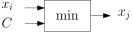
min1v1c

Minimum between a state and a constant.

Syntax

& min1v1c
x_i
x_j
{C}

x_i is the input state, x_j is the output ($\min(x_i, C)$), and C is a constant (data name, parameter name, or math expression).

Internal states: none

Discrete variable: $z \in \{1, 2\}$

Equations

$$0 = \begin{cases} x_j - x_i & \text{if } z = 1 \\ x_j - C & \text{if } z = 2 \end{cases}$$

When $z = 1$ the output tracks $x_i$; when $z = 2$ the output is clamped to $C$.

Discrete transitions

if z = 1:
    if x_i > C:
        z ← 2
else:  # z = 2
    if x_i <= C:
        z ← 1

Initialization

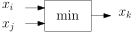
if x_i < C:
    z ← 1
else:
    z ← 2

---

min2v

Minimum between two states.

Syntax

& min2v
x_i
x_j
x_k

x_i and x_j are the two input states; x_k is the output ($\min(x_i, x_j)$).

Internal states: none

Discrete variable: $z \in \{1, 2\}$

Equations

$$0 = \begin{cases} x_i - x_k & \text{if } z = 1 \\ x_j - x_k & \text{if } z = 2 \end{cases}$$

When $z = 1$ the output follows $x_i$; when $z = 2$ the output follows $x_j$.

Discrete transitions

if z = 1:
    if x_i > x_j:
        z ← 2
else:  # z = 2
    if x_j >= x_i:
        z ← 1

Initialization

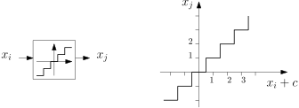
if x_i < x_j:
    z ← 1
else:
    z ← 2

---

nint

Integer nearest to the input shifted by a constant $c$.

Syntax

& nint
x_i
x_j
{c}

x_i is the input state, x_j is the output (nearest integer), and c is a shift constant (data name, parameter name, or math expression).

Internal states: none

Discrete variable: $z \in \mathcal{I}$ (the integers)

Equations

$0 = x_j - z$

Discrete transitions

if nint(x_i + c) ≠ z:
    z ← nint(x_i + c)

where $\text{nint}(\cdot)$ returns the nearest integer.

Initialization

$z \leftarrow \text{nint}(x_i + c)$

Notes, particular cases

• With $c = 0$: the output is the integer nearest to $x_i$.
• With $c = -0.5$: the output is the floor of $x_i$ (largest integer $\le x_i$).
• With $c = 0.5$: the output is the ceiling of $x_i$ (smallest integer $\ge x_i$).

---

pwlin

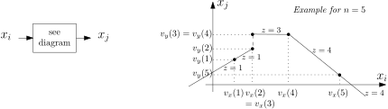
Piece-wise linear function of input, defined by $n$ points. Separate blocks exist for $n = 3, 4, 5$ and $6$.

Syntax

& pwlin3
name of variable x_i
name of variable x_j
data/parameter/expression for v_x(1)
data/parameter/expression for v_y(1)
data/parameter/expression for v_x(2)
data/parameter/expression for v_y(2)
data/parameter/expression for v_x(3)
data/parameter/expression for v_y(3)

For pwlin4, pwlin5, and pwlin6, append additional $(v_x(k), v_y(k))$ pairs up to $k = 4$, $5$, or $6$ respectively.

Internal States

None.

Discrete Variables

$z \in \{1, \ldots, n-1\}$

Equations

$0 = v_y(z) + \frac{v_y(z+1) - v_y(z)}{v_x(z+1) - v_x(z)} \left( x_i - v_x(z) \right) - x_j$

Discrete Transitions

if x_i < v_x(1):
  z ← 1
else if x_i >= v_x(n):
  z ← n-1
else:
  for k = 1 to n-1:
    if v_x(k) <= x_i < v_x(k+1):
      z ← k

Initialization

Same logic as discrete transitions.

Notes

• The $v_x$ values must be strictly increasing at the endpoints: $v_x(1) < v_x(2)$ and $v_x(n-1) < v_x(n)$; intermediate values may be equal: $v_x(1) < v_x(2) \le \cdots \le v_x(n-1) < v_x(n)$.
• For $x_i < v_x(1)$ or $x_i > v_x(n)$, $x_j$ is obtained by linear extrapolation from the first or last two points respectively.

---

See Also

• Block Index, all CODEGEN blocks by category
• CODEGEN Model Examples, complete models built from these blocks
• User-Defined Models, the DSL file format