Eigenanalysis

RAMSES computes small-signal stability analysis internally. It reduces the linearised differential-algebraic model to a state matrix, solves the dense eigenproblem, and writes eigenvalues, damping ratios, participation factors and mode shapes to file. No external tool is involved.

Watch it

Episode 7 of the video series, Small Signal Stability and Eigenanalysis, covers this page.

What is computed

The linearised model is a set of differential-algebraic equations,

\begin{aligned} \Delta\dot{x} &= f_x\,\Delta x + f_y\,\Delta y \\ 0 &= g_x\,\Delta x + g_y\,\Delta y \end{aligned}

with states $x$ and algebraic variables $y$ . Eliminating $\Delta y$ gives the state matrix

$A_{sys} = f_x - f_y\,g_y^{-1}\,g_x$

whose eigenvalues are the system modes. RAMSES assembles the unreduced Jacobian, factorises $g_y$ once with KLU, forms $A_{sys}$ , and solves it with LAPACK. The elimination exists only if $g_y$ is nonsingular, which is what makes the model index-1; a singular $g_y$ is reported rather than worked around.

For each eigenvalue $\lambda = \sigma \pm j\omega$ :

Quantity	Definition
Frequency	$f = \lvert\omega\rvert / 2\pi$ in Hz
Damping ratio	$\zeta = -\sigma / \lvert\lambda\rvert$

A mode with $\zeta < 0$ grows rather than decays: the operating point is small-signal unstable.

Running an analysis

Add an EIG event to the disturbance file:

1.000 EIG 'ssa'

or drive it from Python, which supplies the two solver settings itself:

import stepss
from stepss import ssa

case = stepss.cfg()
case.addData("lf.dat")
case.addData("dyn.dat")
case.addDst("nothing.dst")
case.addObs("obs.dat")
case.addTrj("out.trj")

res = ssa.run(case, basename="ssa")
res.electromechanical().table()
res.electromechanical().splane()

See the stepss.ssa reference for the filters, the participation and mode-shape accessors, and the archive both interfaces exchange.

Results are computed at the instant the event fires, so where you pause determines what you get. Small-signal results are only meaningful at an operating point: pausing mid-swing linearises about a non-equilibrium.

Required settings

Setting	Why
`$OMEGA_REF SYN`	Under the centre-of-inertia frame the COI equations are computed by finite differences and never enter the assembled Jacobian, so reducing under COI would silently hold COI speed constant and produce a plausible, wrong spectrum
`$SCHEME DE`	Under the integrated scheme the pure differential-algebraic values exist only briefly inside the Newton loop

Both are refused rather than approximated. See Refusals below.

One optional setting, $PF_THRES x, sets the floor below which a participation entry is not written, default 1e-3. It is a size guard on the one output that is quadratic in the state count, in the same family as $EIG_MAX_STATES, and not a threshold anyone is meant to tune per analysis; see <name>_pf.dat below.

They are yours to set on the command line and from Python, and ssa.run() above does exactly that, writing both into a generated file read last so the case itself needs no edit for the two settings. The graphical interface’s Run small-signal stability analysis writes both itself, into an extra data file read after the case’s own, so a case configured for time-domain runs analyses without being edited. Settings are applied in the order they are read and the last of each kind wins, which is what makes that an override rather than a conflict.

Output files

Three files per analysis, named from the basename given to EIG, each starting with a # comment header. <name>_modes.dat is numeric throughout, so numpy.loadtxt reads it directly. <name>_pf.dat and <name>_ms.dat also carry a device name, written as the engine stored it rather than justified for splitting, so a name may carry a leading or embedded blank and splitting on whitespace misreads those columns silently. Both are read by fixed column offset instead, and stepss.ssa does this for you.

All three carry every mode. Nothing the engine writes decides which modes are worth looking at; that is the reader’s job, and both interfaces filter live against the full set. The only floor anywhere is $PF_THRES, on participation alone, and its reason is size rather than significance.

The first line of each file is a version banner, and these three are at v2.

`<name>_modes.dat`

One line per mode, every mode written.

Column	Meaning
`index`	Mode number, 1-based
`re`, `im`	Real and imaginary parts of $\lambda$
`zeta`	Damping ratio
`freq_hz`	Frequency in Hz
`smp`	1 if the eigenvalue is simple, 0 if degenerate

The header records nstates, nalg, the time, gap_tol, and pf_floor, the participation floor the run applied.

`<name>_pf.dat`

Participation factors, one line per mode and state: mode, state, pf, family, device, variable. The pf column is the participation factor itself.

The participation of state $k$ in mode $i$ is $p_{ki} = \lvert w_{ki}\,v_{ki}\rvert$ , built from the left and right eigenvectors and normalised so each mode’s largest entry is 1.

Written for every mode, and for every entry above $PF_THRES, so a state that is absent is below that floor rather than exactly zero. This is the one output quadratic in the state count: one row per (mode, state) pair, so at the $EIG_MAX_STATES ceiling of 5000 states an unfloored file would be 25 million rows and roughly 2 GB, nearly all of it entries too small to read. At the default the same run writes on the order of a hundred thousand.

No mode can be emptied by the floor for any value below 1, because normalisation puts one entry at exactly 1 in every mode. Raise it to bound the file on a large system; lower it to see smaller entries.

`<name>_ms.dat`

Mode shapes, one line per mode and machine: mode, state, magnitude, angle_deg, device.

Rotor-speed components for every mode, normalised so the largest magnitude in each mode is 1, with angles relative to that largest entry, because an eigenvector’s absolute phase is arbitrary. No floor applies: this carries one row per machine per mode, which is linear in the state count rather than quadratic.

Saving a run as one archive

The three files above are only useful together, and a spectrum is only worth much beside the matrix it was reduced from. STEPSS GUI writes all of them, plus the Jacobian that the JAC disturbance dumped at the same instant, into a single .zip or .tar.gz: Save dynamic Jacobian… on the Analysis tab, with the format chosen in the dialog. Load dynamic Jacobian… beside it opens one back into a results window of its own, leaving any window already up alone, so an archived run and a fresh one can be read side by side.

In the archive
`stepss-ssa.txt`	The manifest: the basename, the engine version and `t` (older archives also carry the `real_limit` and `pf_threshold` their run was given)
`<name>_modes.dat`, `<name>_pf.dat`, `<name>_ms.dat`	The results above
`<name>_eqs.dat`, `<name>_var.dat`, `<name>_val.dat`, `<name>_struc.dat`	The unreduced Jacobian

An archive is a record of a result, not an input that reproduces one. The data files, the solver settings and the disturbance that produced the run are not in it. It is something to hand to a colleague, attach to an issue, or come back to in a year and still be able to read; re-running the analysis needs the case, which is a separate thing to keep.

The manifest is what makes it readable that much later. None of the results files records which engine wrote them, so an archive analysed by an older build is otherwise indistinguishable from one made today: STEPSS names the recorded version when it opens one, and says so when it differs from the engine now in use. An archive carrying no manifest is refused with a reason rather than opened into an empty window.

Both formats are ordinary archives that unzip and tar xzf read, and everything sits under one directory named for the run. The archive is also the only way back into the interface: results sitting loose in a directory, from a run made at a terminal for instance, are read by ssa.load() rather than by STEPSS GUI, which opens a run either by producing it or by loading one of these.

Degenerate modes, and why the `smp` column matters

Identical machine models with identical parameters produce identical poles, so power system spectra are heavily degenerate. In the Kundur two-area system, 20 of 70 modes share an eigenvalue with another mode.

In a degenerate eigenspace the individual eigenvectors are not unique. The participation factors and mode shape of such a mode are therefore basis-dependent: real numbers that carry no physical meaning and that would come out differently on another LAPACK build.

The smp column is 1 when the gap from this eigenvalue to every other exceeds gap_tol (default 1e-6, recorded in the header), and 0 otherwise. Do not interpret participation factors or mode shapes for a mode flagged 0.

Refusals

The analysis refuses rather than returning a result it cannot justify. Every refusal writes no results files, states the reason in the log and through getLastErr(), and exits with code 78.

Condition	Reason
`$OMEGA_REF COI`	The assembled Jacobian does not carry the COI equations
`$SCHEME IN`	The pure DAE values are not available at that point
States above `$EIG_MAX_STATES`	The dense solve is not practical at that size
Singular $g_y$	The model is not index-1
`EIG` carrying parameters	The record takes a basename and nothing else

That last one is a migration, not a mistake in the usual sense. EIG used to accept an optional real_limit and pf_threshold pair; real_limit decided which modes got participation and mode-shape output, and pf_threshold became the $PF_THRES solver setting. A .dst still carrying them is refused rather than having them ignored, because the values changed what the old engine wrote and accepting one silently would produce a results set that looks entirely normal and answers a different question. Remove the parameters; if you want the old participation floor, write $PF_THRES 0.05 ; in your solver settings.

A run that produced nothing and exited 0 is a different problem, most likely an engine older than v3.60.

The size ceiling is $EIG_MAX_STATES, default 5000. Systems beyond it need sparse shift-invert methods, which scipy.sparse.linalg.eigs can drive from the descriptor matrices getJac() returns.

Worked example

The Kundur two-area system is the standard inter-area oscillation benchmark, and the stepss package ships an annotated notebook for it under examples/eigenanalysis/. Analysed with and without its power system stabilisers:

	inter-area	area 1 local	area 2 local
without PSS	0.625 Hz, $\zeta$ = -0.0233	1.085 Hz, $\zeta$ = 0.099	1.116 Hz, $\zeta$ = 0.097
with PSS	0.624 Hz, $\zeta$ = +0.1087	1.242 Hz, $\zeta$ = 0.288	1.295 Hz, $\zeta$ = 0.287

The inter-area damping ratio flips sign with the stabilisers: without them the 0.62 Hz oscillation between the two areas grows and the operating point is small-signal unstable. This reproduces Kundur, Power System Stability and Control, Example 12.6.

Participation factors separate the two local modes without any prior knowledge of the topology: the 1.085 Hz mode lists only G1 and G2, the 1.116 Hz mode only G3 and G4, and the inter-area mode lists all four.

Every one of those numbers is available for every mode, which was not always true: the engine used to write participation factors and mode shapes only for modes above a real_limit fixed before the run, so answering a question about a mode outside it meant running the case again.

In STEPSS GUI the same run is read from the small-signal results window, which Run small-signal stability analysis on the Analysis tab opens on the run it just made:

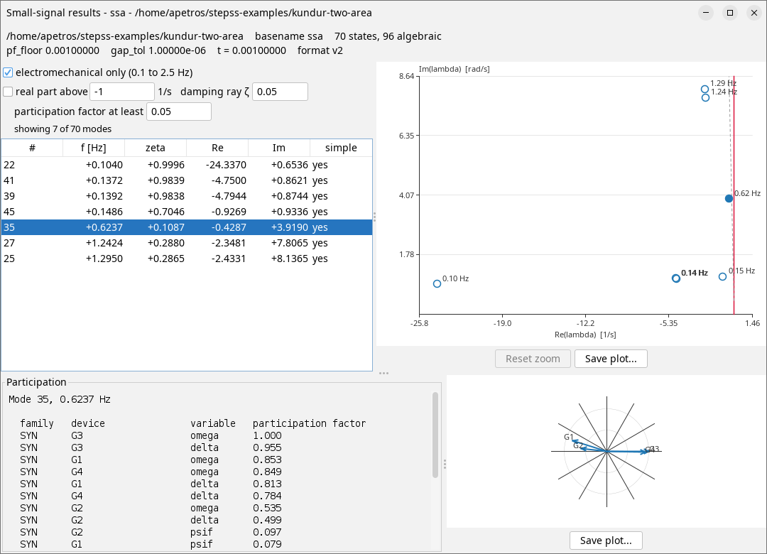
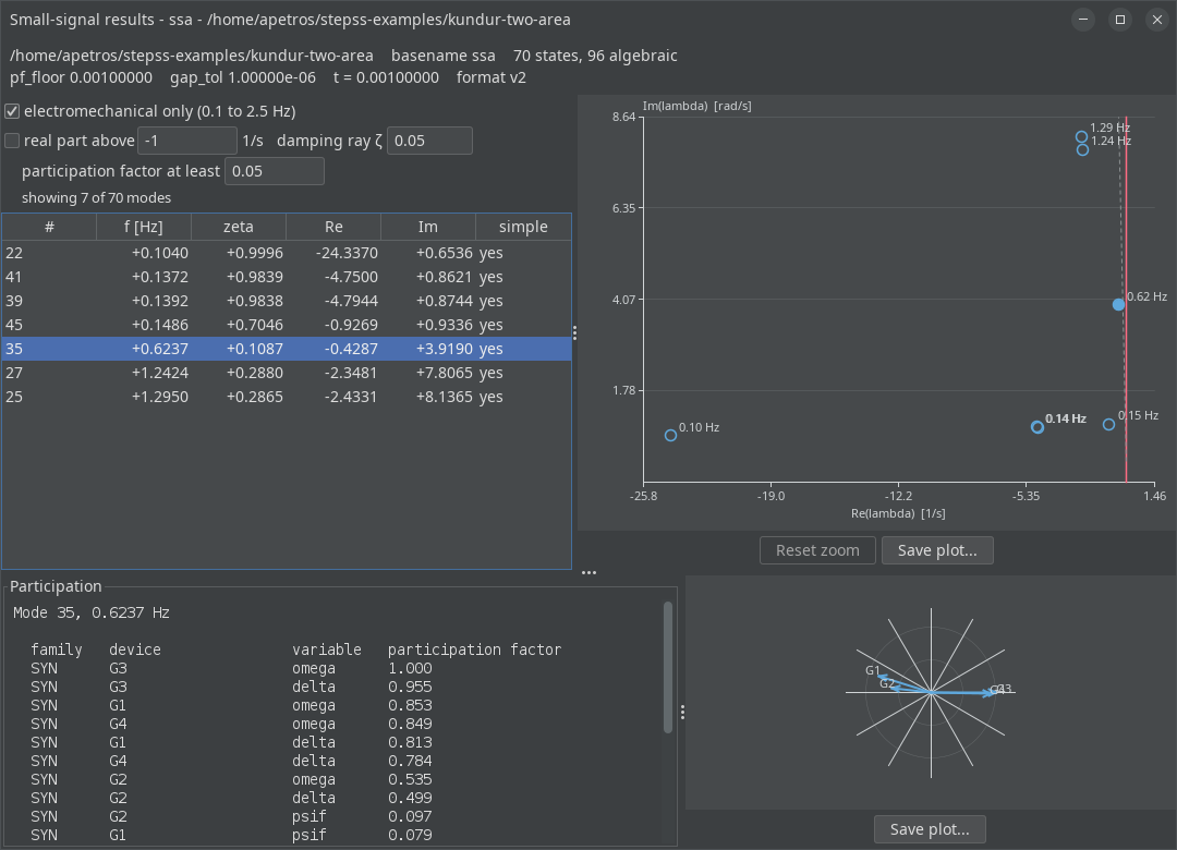
Reading that window across is the whole method in one view. The table gives the frequency and damping of each mode; the s-plane shows how much margin each one has, with the boundary drawn at the imaginary axis, so a mode crossing it is the instability. Every mode is one circle there, crimson if it is unstable and filled if it is the one selected. The dashed line beside the boundary is a constant-damping ray, described below. The Participation panel answers which machines make up that mode, its last column giving the participation factor, normalised so the largest in each mode is 1. The mode shape answers how those machines move relative to each other: here G1 and G2 swing against G3 and G4, which is what makes 0.62 Hz the inter-area mode rather than a local one.

Filtering and zooming

Four controls sit above the table, and all of them act on results already in hand. None requires the analysis to be run again.

Control	What it does
electromechanical only	Restricts to the 0.1 to 2.5 Hz band, where rotor-angle modes live. On by default
real part above	Hides modes at or below the value beside it. Off by default
damping ray $\zeta$	Moves the dashed ray on the s-plane to another damping ratio. A display option: it hides nothing
participation factor at least	Trims the Participation panel to entries at or above the value beside it

The count underneath says how many modes survive, so a filter that empties the table reads as a filter rather than as a broken load.

real part above is the one that used to be the real_limit parameter of the run. It is worth reaching for on a full spectrum: this case is 70 states, most of them fast controller and network dynamics that no rotor participates in, and a handful of them sit far enough to the left to stretch the s-plane’s real axis until everything worth reading is squashed against the boundary. The plot refits its axes whenever the filter changes, so hiding those modes closes the plane in around what is left.

The fitted window always contains the origin, whatever the modes do, so the imaginary axis and the foot of the damping ray are in every picture and two runs of different systems can be compared by eye.

For a closer look than a filter gives, drag a rectangle on the s-plane to zoom into it. A zoom is yours and is not widened back to the origin. Reset zoom, beside Save plot…, goes back to the fitted window, and double-clicking the plot does the same. A zoomed plot exports zoomed: Save plot… writes what is on screen, not the whole plane.

The damping ray

The dashed line running up beside the stability boundary is a line of constant damping ratio. It leaves the origin at $\arcsin\zeta$ from the imaginary axis, so a mode to the left of it is better damped than that $\zeta$ and a mode to the right is worse. Because $\zeta$ is a ratio rather than a distance, the real part a mode is allowed grows with its frequency, which is exactly what the slant encodes: a 1.7 Hz mode has to sit further left than a 0.35 Hz one to reach the same damping.

It is drawn at 0.05 by default, the usual planning criterion, and the box beside real part above moves it. Type any value from 0 up to (but not including) 1; anything else is refused and the box returns to what it was.