

Running a Simulation
This walks one case end to end: the Kundur two-area system, a load step, and the inter-area oscillation that follows. It needs no data of your own, because the case ships with the application.
If you have not opened it yet, First Run covers File, Open Examples. Pick Kundur two-area and come back.
Watch it
Section titled “Watch it”Episode 5 of the video series, Observables, Trajectories and Plotting, covers this page.
1. Check what was loaded
Section titled “1. Check what was loaded”Opening the example fills the case in, so there is nothing to do here but look. System Data should hold three system data files and one disturbance file:
| Slot | File | What it holds |
|---|---|---|
| System data 1 | lf.dat | The network and the power-flow data |
| System data 2 | dyn.dat | The dynamic models: machines, exciters, governors, loads |
| System data 3 | solveroptions.dat | Solver settings |
| Disturbance | disturb.dst | What happens, and when |
The disturbance is three lines, and worth reading before running anything:
0.000 CONTINUE SOLVER BD 0.01 0.0001 0. ALL 1.000 CHGPRM INJ L9 Po +0.5 0 60.000 STOPAt t = 1 s the active power set point of load L9 is stepped by +0.5 pu, and
the run ends at 60 s. Disturbances is the reference
for these records.
2. Choose what to record
Section titled “2. Choose what to record”On Observables, obs.dat is already loaded and Save output trajectory is
already checked, which is the pair you need: the trajectory is the file the curves
come from, and the observables file says what goes into it.
If you want to watch the run as it happens, set a runtime observable. Machine
speed of G1 and the voltage of bus 9 are good choices for this case. A refresh
interval of 1 second is plenty.
3. Solve the power flow
Section titled “3. Solve the power flow”On Power Flow Simulation, click Run power flow.
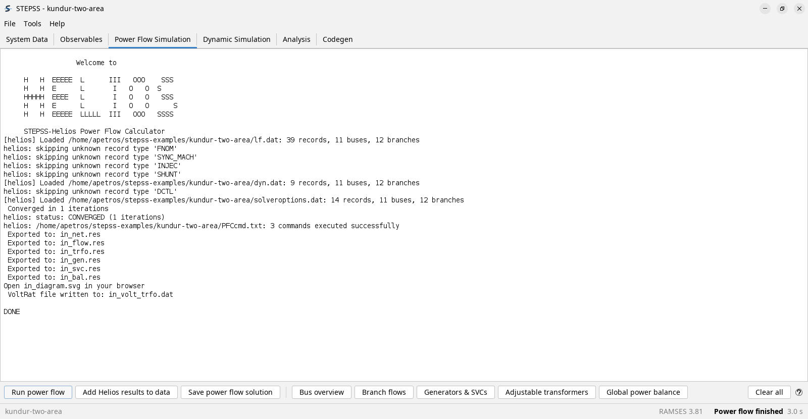
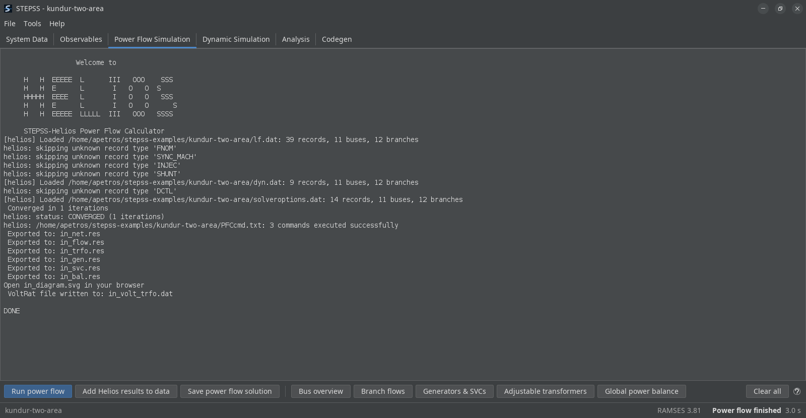
Read the balance at the bottom before going on. For this case the load totals 2734 MW against 2819 MW of generation, the difference being the 85.1 MW of network losses. A balance that does not add up, or a generator sitting on a reactive limit, is a problem to fix here rather than to discover halfway through a dynamic run.
The five inspection buttons beside Run power flow become available now: Bus overview, Branch flows, Generators & SVCs, Adjustable transformers and Global power balance, each of which writes its table into the same pane. The Interface shows what each one produces.
4. Run the simulation
Section titled “4. Run the simulation”On Dynamic Simulation, click Run dynamic simulation.
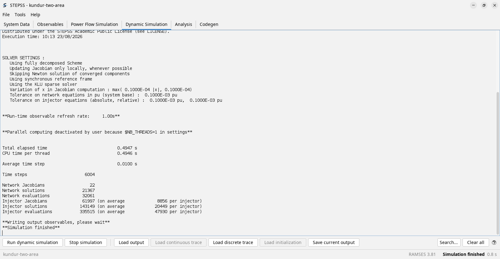
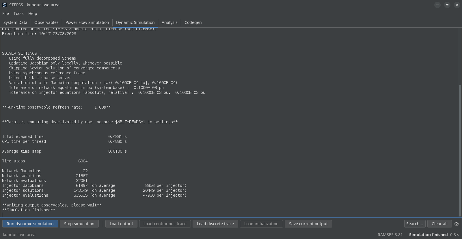
The pane opens with the settings actually in force, which is the place to confirm that the case is doing what you meant. This one reports the synchronous reference frame, the KLU sparse solver, local Jacobian updates, and that converged components are skipped.
It also says parallel computing deactivated by user, because the case sets
$NB_THREADS 1. That is a property of this example, not a limit of the engine.
60 seconds of system time takes well under a second of wall time here, in 6004 steps. The counts below are the cost of the run: how often the network and the injector Jacobians were rebuilt and solved. They are what to watch when a bigger case gets slow.
If you set the runtime observables in step 2, a Run-time curves window drew them as the run advanced and is still up when it finishes; see Real-time plotting.
5. Extract the curves
Section titled “5. Extract the curves”On Analysis, click Extract curves. The picker reads the trajectory and offers whatever the observables file recorded.
-
Set Category to
SYNC, which lists the four synchronous machines. -
Select
G1and set Observable toactive power produced (MW), then click Add. -
Select
G3, leave the observable as it is, and Add again. -
Click Plot.
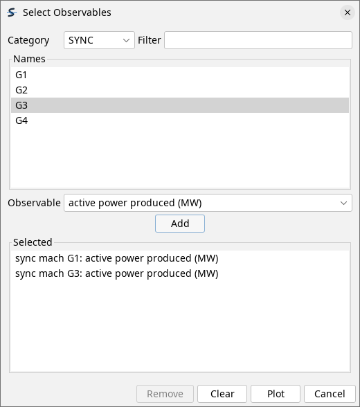
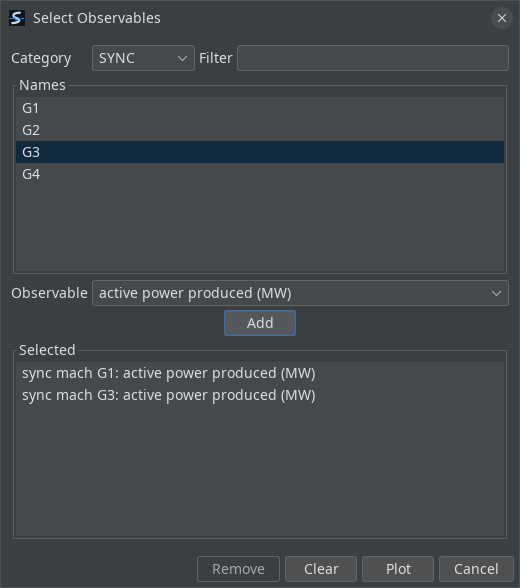
G1 and G3 are the point of the exercise: one sits in each area, so putting them
on the same axes shows the oscillation between the areas rather than within one.
6. Read the result
Section titled “6. Read the result”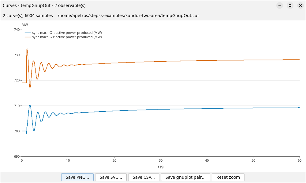
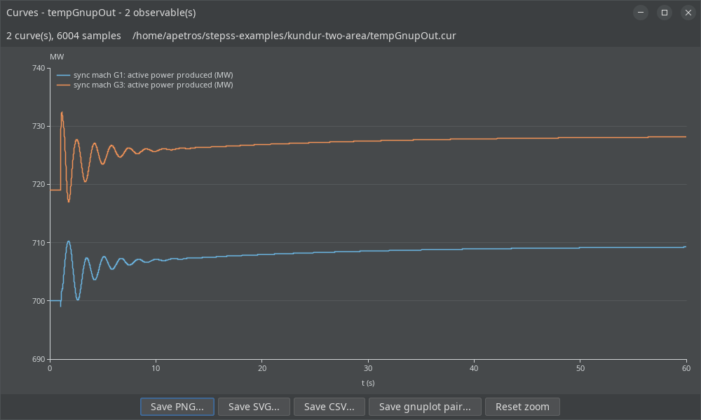
Three things to see in it.
The two machines swing in opposition. When G3 is at a peak, G1 is near a
trough. That anti-phase pattern is what makes this an inter-area mode rather than a
local one: the two areas are oscillating against each other across the weak tie.
The period is about 1.4 seconds, so roughly 0.7 Hz, which is the range inter-area modes normally sit in.
The oscillation decays, and after about ten seconds both machines settle a few megawatts above where they began, sharing the extra load. That decay is the damping, and it is the quantity the next section changes.
Try it with the stabiliser out
Section titled “Try it with the stabiliser out”The example ships a second dynamic file, dyn_noPSS.dat, identical to dyn.dat
except that the power system stabiliser gain is set to zero.
On System Data, load dyn_noPSS.dat into slot 2 in place of dyn.dat, then
repeat steps 3 to 6. Everything else stays as it is.
The mode is the same and its frequency barely moves, but it is far less damped. Comparing the two runs is the standard demonstration of what a PSS is for, and it is why the case ships both files.
Where to go next
Section titled “Where to go next”- Disturbances, to change what happens and when
- Solver Settings, to change how it is solved
- Eigenanalysis, to get this mode’s frequency and damping as numbers instead of reading them off a curve
- Kundur Two-Area System, the system itself in detail
- STEPSS in Python, the same run as a script