Frequency Estimation Blocks

Blocks that expose the frequency RAMSES estimates at the bus a device is connected to. Which block to use depends on the model type.

---

f_inj

Computes $f$, an estimate of the frequency (in per unit) at a given bus, from the evolution of the rectangular components $v_x$ and $v_y$ of the bus voltage. A measurement time constant $T$ is involved. Can be used in the model of an injector only.

Syntax

& f_inj
f
{T}

f is the name of the estimated frequency variable; T is the measurement time constant (data name, parameter name, or math expression). The voltage components $v_x$ and $v_y$ are automatically inherited and must not be declared.

Internal states: $v_{xm}$ and $v_{ym}$ (measured/filtered voltage components)

Discrete variables: none

Equations

$$\begin{aligned} \dot{v}_{xm} &= \frac{v_x - v_{xm}}{T} \\[6pt] \dot{v}_{ym} &= \frac{v_y - v_{ym}}{T} \\[6pt] 0 &= \omega_{ref,pu} + \frac{(v_y - v_{ym})\,v_{xm} - (v_x - v_{xm})\,v_{ym}}{2\pi f_N T \left(v_{xm}^2 + v_{ym}^2\right)} - f \end{aligned}$$

Initialization

$v_{xm} = v_x \qquad v_{ym} = v_y$

Explanation

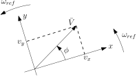
The voltage components $v_x$ and $v_y$ are the projections of the bus voltage phasor onto the reference axes rotating at angular speed $\omega_{ref}$ (rad/s). The instantaneous angular frequency is:

$\omega = \omega_{ref} + \frac{d\phi}{dt}, \qquad \phi = \arctan\frac{v_y}{v_x}$

The per-unit frequency is therefore:

$f = \frac{\omega}{2\pi f_N} = \omega_{ref,pu} + \frac{1}{2\pi f_N}\frac{d}{dt}\!\left(\arctan\frac{v_y}{v_x}\right) = \omega_{ref,pu} + \frac{1}{2\pi f_N}\frac{\dot{v}_y v_x - \dot{v}_x v_y}{v_x^2 + v_y^2}$

where $f_N$ is the nominal frequency (known from the system data). To filter transients, $v_x$ and $v_y$ are passed through first-order filters with time constant $T$, yielding the measured values $v_{xm}$ and $v_{ym}$. Substituting the filter derivatives into the frequency expression yields the third equation above.

Notes

• A recommended value for $T$ is in the range $0.05$–$0.10$ s.
• $T = 0$ is not allowed. If $T$ is too small, the solver may encounter a singularity and the simulation may fail.

---

f_twop_bus1

Similar to f_inj. Computes $f$, an estimate of the frequency (in per unit) at the first bus of a given two-port. Can be used in the model of a two-port only.

Syntax

& f_twop_bus1
f
{T}

f is the name of the estimated frequency variable; T is the measurement time constant (data name, parameter name, or math expression).

Internal states: $v_{xm}$ and $v_{ym}$ (filtered voltage components at bus 1)

Discrete variables: none

Equations, initialization, and notes: identical to f_inj, refer to that block for the full mathematical description. The only difference is that this block uses the voltage at the first bus of a two-port rather than an injector bus.

---

f_twop_bus2

Similar to f_inj. Computes $f$, an estimate of the frequency (in per unit) at the second bus of a given two-port. Can be used in the model of a two-port only.

Syntax

& f_twop_bus2
f
{T}

f is the name of the estimated frequency variable; T is the measurement time constant (data name, parameter name, or math expression).

Internal states: $v_{xm}$ and $v_{ym}$ (filtered voltage components at bus 2)

Discrete variables: none

Equations, initialization, and notes: identical to f_inj, refer to that block for the full mathematical description. The only difference is that this block uses the voltage at the second bus of a two-port rather than an injector bus.

---

See Also

• Block Index, all CODEGEN blocks by category
• CODEGEN Model Examples, complete models built from these blocks
• User-Defined Models, the DSL file format