Automata & Timer Blocks

Blocks driven by discrete logic rather than differential equations: automata that switch on signal conditions, and timers that fire after a delay.

---

fsa

Finite State Automaton.

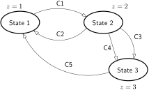
This block forces a set of $n$ algebraic equations. There are $s$ possible sets, each corresponding to a value of the discrete state $z$. Transitions between sets occur when Boolean expressions evaluate to true.

Syntax

The block is specified via an inline example. For $s = 3$ states and $n = 2$ algebraic constraints per state:

& fsa
initial_state
# 1
algebraic constraint No. 1
algebraic constraint No. 2
-> 2
boolean expression C1
# 2
algebraic constraint No. 3
algebraic constraint No. 4
-> 1
boolean expression C2
-> 3
boolean expression C3
-> 3
boolean expression C4
# 3
algebraic constraint No. 5
algebraic constraint No. 6
-> 1
boolean expression C5
##

Internal states: none

Discrete variable: $z$. The index of the currently active state

Syntax rules

Token	Meaning
# N	Begins the section for state $N$. States must be numbered consecutively from 1 to $s$ in increasing order.
##	Marks the end of the state list.
-> N	Declares a transition to state $N$. The following line is the Boolean expression that triggers the transition.
Second line	Integer specifying the initial state of the automaton.

Notes

• The number $n$ of algebraic constraints must be identical across all states.
• Multiple transitions from the same state to the same target state are permitted (e.g., two separate conditions C3 and C4 both targeting state 3 in the example). Alternatively a single transition with the combined condition C3 or C4 may be used.
• Transitions and algebraic constraints may involve any model states and parameters.

---

tsa

Two-state automaton with transitions based on signs of two inputs.

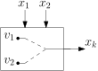
The output state $x_k$ can take two values: $v_1$ or $v_2$. When $x_k = v_1$, a positive $x_1$ triggers the transition to $v_2$; when $x_k = v_2$, a positive $x_2$ triggers the return to $v_1$.

Syntax

& 2sa
name of variable x_1   (trigger for transition to v_2)
name of variable x_2   (trigger for transition to v_1)
name of variable x_k   (output)
data/parameter/expression for v_1
data/parameter/expression for v_2

Internal States

None.

Discrete Variables

$z \in \{1, 2\}$ represents the automaton state.

Equations

$$0 = \begin{cases} x_k - v_1 & \text{if } z = 1 \\ x_k - v_2 & \text{if } z = 2 \end{cases}$$

Discrete Transitions

if z = 1 and x_1 > 0:  z ← 2
else if z = 2 and x_2 > 0:  z ← 1

Initialization

$z \leftarrow 1 \quad (x_k = v_1 \text{ is assumed initially})$

---

timer

Timer with varying delay. The delay is a piecewise linear function of the monitored variable. Separate blocks exist for $n = 1, 2, 3, 4, 5$ and $11$ characteristic points, named timer1 to timer5 and timer11.

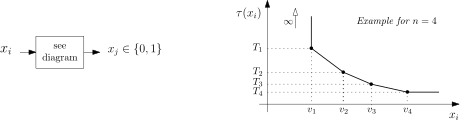
If $x_i$ is smaller than a threshold $v_1$, the output $x_j$ is zero. Otherwise, $x_j$ changes from zero to one at time $t^\star + \tau(x_i)$, where $t^\star$ is the time at which $x_i$ first exceeded $v_1$ and $\tau(x_i)$ is a piecewise linear function of $x_i$ defined by the $(v_k, T_k)$ pairs.

Syntax

& timer1
name of variable x_i
name of variable x_j
data/parameter/expression for v_1
data/parameter/expression for T_1

For timer2 to timer5, append additional $(v_k, T_k)$ pairs up to the required $n$. timer11 takes 11 pairs (22 parameters).

Internal States

$x_1$ (elapsed time counter)

Discrete Variables

$z \in \{-1, 0, 1\}$

Equations

$$0 = \begin{cases} x_j & \text{if } z \in \{-1, 0\} \\ x_j - 1 & \text{if } z = 1 \end{cases}$$ $$\begin{cases} 0 = x_1 & \text{if } z = -1 \\ \dot{x}_1 = 1 & \text{if } z = 0 \\ \dot{x}_1 = 0 & \text{if } z = 1 \end{cases}$$

Discrete Transitions

if z = -1:
  if x_i >= v_1:  z ← 0
else (z = 0 or 1):
  if x_i < v_1:  z ← -1

if z = 0:
  if x_1 >= τ(x_i):  z ← 1

Initialization

$x_1 \leftarrow 0, \qquad z \leftarrow -1$

Notes

• The $v_i$ values must be non-decreasing: $v_1 \le v_2 \le \cdots \le v_n$.
• Typical use: approximating an inverse-time characteristic with $T_1 \ge T_2 \ge \cdots \ge T_n$.
• Non-decreasing $T$ values are also allowed (i.e., $T_1 \le T_2$ is permitted).
• If $x_i > v_1$ at $t = 0$, $x_j$ will trip to one after $\tau(x_i)$ unless $x_i$ drops below $v_1$ first.

---

timersc

Timer with varying delay. The delay is a staircase function of the monitored variable. Separate blocks exist for $n = 1, 2, 3, 4, 5$ and $6$ characteristic points.

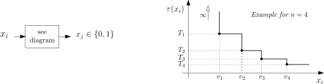
Identical behaviour to timer except that the delay function $\tau(x_i)$ is a staircase (step) function instead of a piecewise linear interpolation.

Syntax

& timersc1
name of variable x_i
name of variable x_j
data/parameter/expression for v_1
data/parameter/expression for T_1

For timersc2–timersc6, append additional $(v_k, T_k)$ pairs up to the required $n$.

Internal States

$x_1$ (elapsed time counter)

Discrete Variables

$z \in \{-1, 0, 1\}$

Equations

$$0 = \begin{cases} x_j & \text{if } z \in \{-1, 0\} \\ x_j - 1 & \text{if } z = 1 \end{cases}$$ $$\begin{cases} 0 = x_1 & \text{if } z = -1 \\ \dot{x}_1 = 1 & \text{if } z = 0 \\ \dot{x}_1 = 0 & \text{if } z = 1 \end{cases}$$

Discrete Transitions

if z = -1:
  if x_i >= v_1:  z ← 0
else (z = 0 or 1):
  if x_i < v_1:  z ← -1

if z = 0:
  if x_1 >= τ(x_i):  z ← 1

Initialization

$x_1 \leftarrow 0, \qquad z \leftarrow -1$

Notes

• The $v_i$ values must be non-decreasing: $v_1 \le v_2 \le \cdots \le v_n$.
• The staircase characteristic is typically used to approximate an inverse-time protection curve.
• Non-decreasing $T$ values are also allowed.
• If $x_i > v_1$ at $t = 0$, $x_j$ trips to one after $\tau(x_i)$ unless $x_i$ drops below $v_1$ first.

---

See Also

• Block Index, all CODEGEN blocks by category
• CODEGEN Model Examples, complete models built from these blocks
• User-Defined Models, the DSL file format