Examples

All examples assume the working directory contains the relevant data and disturbance files.

Running a Basic Simulation

Define the test case, run the simulation, and extract results:

import stepss

case = stepss.cfg()
case.addData('dyn_A.dat')        # dynamic models
case.addData('volt_rat_A.dat')   # power-flow initialisation
case.addData('settings1.dat')    # solver settings
case.addDst('short_trip_branch.dst')
case.addInit('init.trace')
case.addTrj('output.trj')        # save trajectories for post-processing
case.addObs('obs.dat')           # define which observables to record
case.addCont('cont.trace')
case.addDisc('disc.trace')
case.addRunObs('BV 4044')        # record bus voltage while the run proceeds
case.addRunObs('BV 1041')
case.writeCmdFile('cmd.txt')     # save for future reuse

ram = stepss.sim()
ram.execSim(case)                # run to completion

ext = stepss.extractor(case.getTrj())
ext.getBus('1041').mag.plot()    # voltage magnitude at bus 1041

Note

Set $NB_THREADS 0 ; in the solver settings file to use all available CPU cores for parallel simulation. The free version uses at most 2 cores whatever this is set to; a $LICENSE record in the data files lifts the cap. See License.

Pause and Continue

Pause the simulation at intermediate time points to inspect state or add disturbances:

ram = stepss.sim()
ram.execSim(case, 0.0)                        # initialise, paused at t=0
ram.contSim(10.0)                             # simulate to t=10 s
ram.contSim(ram.getSimTime() + 60.0)          # advance 60 s from current time
ram.contSim(ram.getInfTime())                 # run to end of time horizon

Querying System State

Query bus voltages, branch flows, observables, and parameters while paused:

ram.execSim(case, 10.0)

# Bus voltages
busNames = ['g1', 'g2', 'g3']
voltages = ram.getBusVolt(busNames)   # list of voltage magnitudes (pu)
phases   = ram.getBusPha(busNames)    # list of phase angles (deg)

# Branch power flows
branch_pq = ram.getBranchPow(['1041-01'])  # [[P_from, Q_from, P_to, Q_to]]

# Component observables: P of injector L_11, vf of exciter g2, Pm of governor g3
comp_type = ['INJ',  'EXC', 'TOR']
comp_name = ['L_11', 'g2',  'g3']
obs_name  = ['P',    'vf',  'Pm']
obs = ram.getObs(comp_type, comp_name, obs_name)

# Component parameters: V0 of exciter g1, KPSS of exciter g2
comp_type = ['EXC', 'EXC']
comp_name = ['g1',  'g2']
prm_name  = ['V0',  'KPSS']
prms = ram.getPrm(comp_type, comp_name, prm_name)

# All component names of a type
all_buses = ram.getAllCompNames('BUS')
all_gens  = ram.getAllCompNames('SYNC')

Adding Disturbances at Runtime

Inject disturbances and parameter changes while the simulation is running:

ram.execSim(case, 80.0)

# LTC voltage setpoint changes at t=100 s (ramp)
for i in range(1, 6):
    ram.addDisturb(100.0, f'CHGPRM DCTL {i}-104{i}  Vsetpt -0.05 0')

# Fault and clearance
ram.addDisturb(100.0, 'FAULT BUS 4032 0. 0.')         # 3-phase short circuit
ram.addDisturb(100.1, 'CLEAR BUS 4032')                # clear fault
ram.addDisturb(100.1, 'BREAKER BRANCH 4032-4044 0 0')  # trip line

# Generator trip
ram.addDisturb(100.0, 'BREAKER SYNC_MACH g7 0')

ram.contSim(ram.getInfTime())

For full disturbance syntax, see the Disturbances reference.

Plotting Results

Extract and plot time-series results after the simulation:

import stepss
ext = stepss.extractor('output.trj')

# Single curve
ext.getSync('g5').S.plot()       # rotor speed of generator g5
ext.getBus('4044').mag.plot()    # voltage magnitude at bus 4044

# Multiple curves on the same plot
curves = [ext.getSync(f'g{i}').S for i in range(1, 5)]
stepss.curplot(curves)

# Exciter and governor outputs
ext.getExc('g1').vf.plot()       # field voltage
ext.getTor('g1').Pm.plot()       # mechanical power

# Branch power flows
ext.getBranch('1041-01').PF.plot()

# Injector (wind/PV/BESS)
ext.getInj('WT1a').Pw.plot()

# Two-port (HVDC)
ext.getTwop('hvdc1').P1.plot()

Every one of those calls opens a matplotlib figure. Run against the bundled Kundur two-area example, whose disturbance steps load L9 at t = 1 s, the first three look like this.

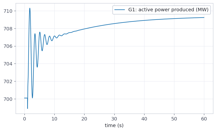
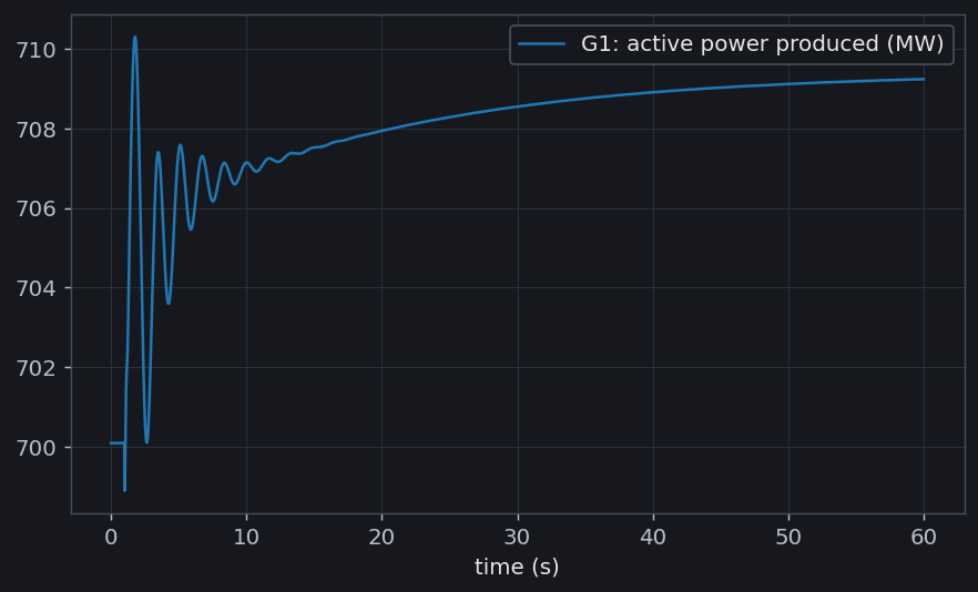
ext.getSync('G1').P.plot(), one curve, labelled from the trajectory:

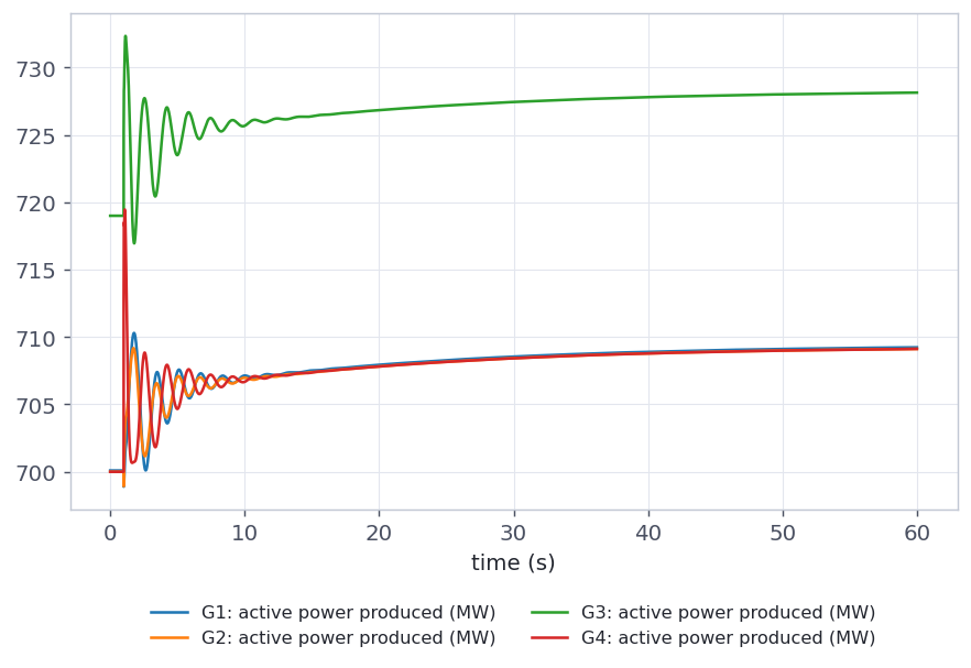
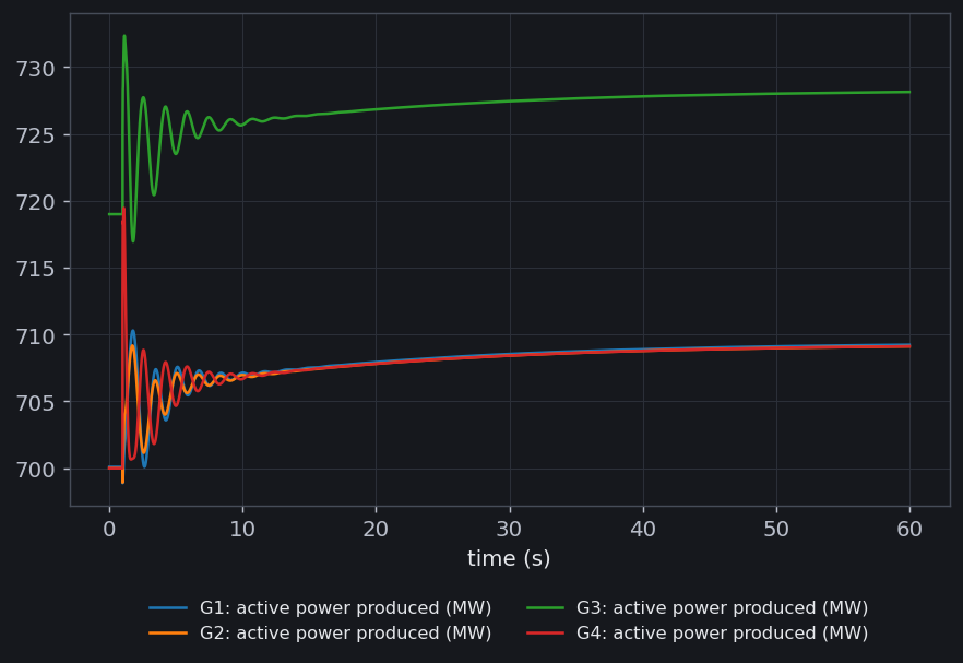
stepss.curplot([...]), several curves on one set of axes. Putting all four machines together is what separates the areas: G3 starts 19 MW above the rest and stays there, while G1, G2 and G4 sit on top of one another.

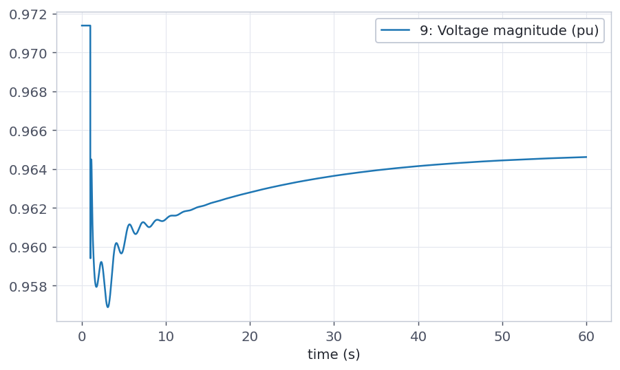
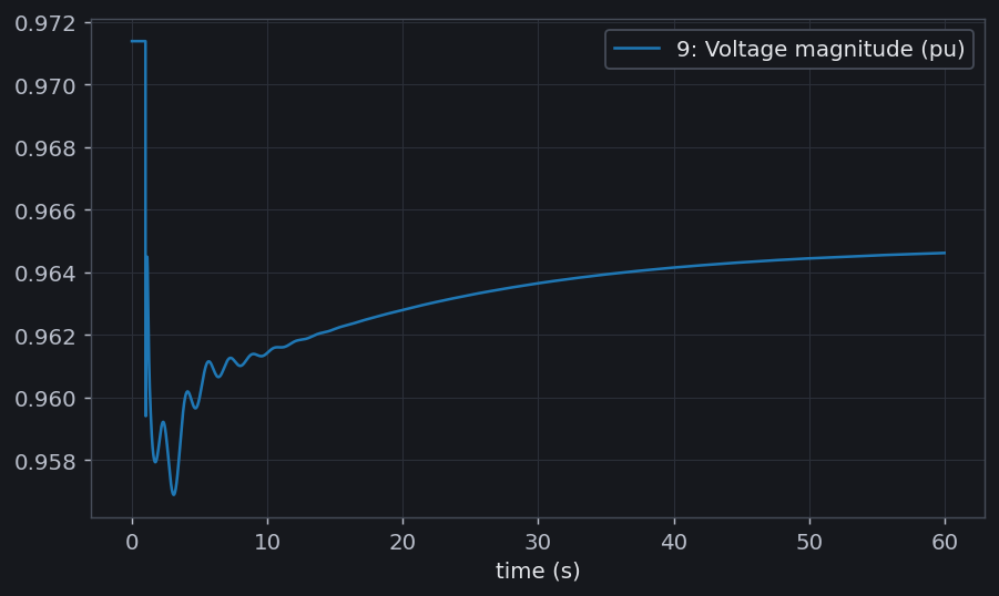
ext.getBus('9').mag.plot(), the same run seen as a voltage rather than a power:

These are ordinary matplotlib figures, so the usual savefig, styling and subplot handling all apply to them.

Live Plotting

Watch chosen quantities as the simulation computes them, one panel per observable:

import stepss

ram = stepss.sim()
ram.execSim(case, 0.0)                   # initialise, paused at t = 0

mon = stepss.monitor(ram, [
    'BV 4044',                           # voltage magnitude of bus 4044
    'MS g6',                             # rotor speed of machine g6
    'BPO 4041-4044',                     # active power at the branch origin
    'RT RT',                             # wall clock, to gauge simulation speed
], title='Nordic')

curves = mon.run(step=0.1)               # to the end of the scenario
mon.savefig('live.png')

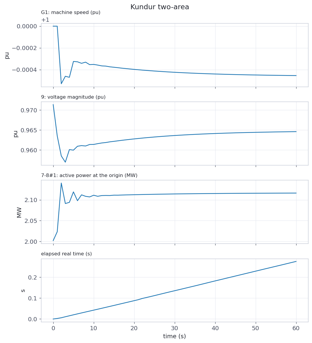
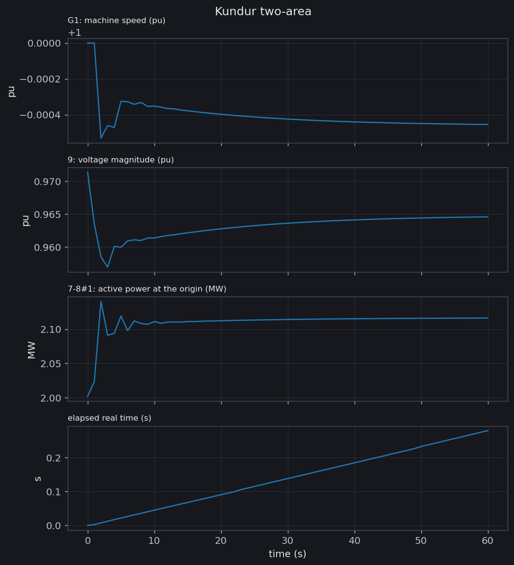
Each observable gets a panel, the panels share the time axis, and the figure is redrawn as the run advances. RT RT is the one to include when you want to see how fast the run itself is going: a straight line means the engine is keeping a steady pace, and a knee in it is where the case got expensive.

run returns the same cur objects the extractor produces, so the collected data goes straight into the post-processing above:

stepss.curplot(curves)

Drive the stepping yourself when the run needs disturbances injected along the way:

mon = stepss.monitor(ram, ['BV 4044', 'BV 1041'])
for target in range(10, 200, 10):
    ram.contSim(float(target))
    mon.sample()
    mon.refresh()
    if target == 100:
        ram.addDisturb(105.0, 'CHGPRM DCTL 1-1041 Vsetpt -0.05 0')

Parameter Sweep

Run multiple simulations with varying parameters and collect results:

import stepss
import numpy as np

results = {}
for disturbance_time in [5.0, 10.0, 20.0]:
    case = stepss.cfg('cmd.txt')
    trj_file = f'output_{disturbance_time:.0f}.trj'
    case.addTrj(trj_file)
    case.addObs('obs.dat')

    ram = stepss.sim()
    ram.execSim(case, 0.0)
    ram.addDisturb(disturbance_time, 'BREAKER SYNC_MACH g7 0')
    ram.contSim(ram.getInfTime())
    ram.endSim()

    ext = stepss.extractor(trj_file)
    min_freq = np.min(ext.getSync('g5').S.value)
    results[disturbance_time] = min_freq
    print(f't_dist={disturbance_time:5.1f}s  min_speed={min_freq:.5f} pu')

Eigenanalysis Workflow

RAMSES performs the small-signal analysis itself, and stepss.ssa drives it, reads its three output files and plots them. One call runs the analysis at the operating point:

import stepss
from stepss import ssa

case = stepss.cfg('cmd.txt')
res = ssa.run(case, basename='ssa', workdir='run1')
res.summary()

ssa.run() copies the case rather than modifying it, supplies the two solver settings the analysis requires, clears any previous run under the same basename, and returns the results.

Filtering happens on the results you already have, so widening a limit costs nothing:

em = res.electromechanical()      # the rotor band, 0.1 to 2.5 Hz
em.table()                        # index, frequency, damping ratio, lambda

res.dominant(-1.0).table()        # the modes above a real part limit

Reading one mode, and plotting:

mode = res.electromechanical(0.4, 0.9)[0]        # the inter-area mode
print('%.4f Hz, zeta = %+.4f' % (mode['freq'], mode['zeta']))

for row in res.participation(mode, floor=0.05):  # which states take part
    print('  %-8s %-8s %.3f' % (row.device.strip(), row.variable, row.pf))

em.splane()                                      # the conventional summary plot
res.mode_shape_plot(mode)                        # the rotor-speed dial

Each plot takes and returns an Axes, so two runs go side by side in one figure. A complete annotated walkthrough ships with the package under examples/eigenanalysis/.

Results made anywhere else are read the same way, including a .ssa archive saved from the graphical interface:

res = ssa.load('run1', 'ssa')                    # three files on disk
res, manifest = ssa.load_archive('kundur.ssa.zip')

To drive your own solver instead, getJac() returns the descriptor-form pair as SciPy sparse matrices. This is the route for systems above $EIG_MAX_STATES, where the engine’s dense solve is not practical and sparse shift-invert methods are needed:

ram = stepss.sim()
ram.execSim(case, 0.0)
A, E = ram.getJac()   # scipy.sparse.csc_matrix
ram.endSim()

Note

The analysis needs $OMEGA_REF SYN ; and $SCHEME DE ;. ssa.run() supplies both itself, in a generated file read after the case’s own data files, so a case of your own needs no edit. A run driven by hand still needs them: EIG refuses without them, exiting 78 with the reason in the log, and the JAC export skips with a warning under COI. See Eigenanalysis and the stepss.ssa reference.

Test System Examples

The following examples use the ready-to-run test systems. For system descriptions, data files, and disturbance scenarios, see the Test Systems section.

Nordic Test System: Generator Trip

Trips generator g7 at $t = 10$ s on the heavily-stressed Operating Point B and observes the voltage collapse dynamics over 150 seconds. See the Nordic Test System page for full system details and file descriptions.

import stepss
import os

case = stepss.cfg()
case.addData('dyn_B.dat')
case.addData('volt_rat_B.dat')
case.addData('settings1.dat')
case.addDst('nothing.dst')
case.addObs('obs.dat')
case.addTrj('output.trj')

for f in os.listdir('.'):
    if f.endswith('.trj') or f.endswith('.trace'):
        os.remove(f)

ram = stepss.sim()
ram.execSim(case, 0.0)
ram.addDisturb(10.0, 'BREAKER SYNC_MACH g7 0')
ram.contSim(150.0)
ram.endSim()

ext = stepss.extractor(case.getTrj())
ext.getSync('g7').S.plot()    # rotor speed
ext.getBus('1041').mag.plot()  # voltage at central bus

5-Bus System: Exciter Parameter Change

Applies a step change to the exciter voltage setpoint at $t = 1$ s and plots the generator response. See the 5-Bus Test System page for details.

import stepss
import os

case = stepss.cfg()
case.addData('dyn.dat')
case.addData('lf1solv.dat')
case.addData('solveroptions.dat')
case.addDst('nothing.dst')
case.addObs('obs.dat')
case.addTrj('output.trj')

for f in os.listdir('.'):
    if f.endswith('.trj') or f.endswith('.trace'):
        os.remove(f)

ram = stepss.sim()
ram.execSim(case, 0.0)
ram.addDisturb(1.0, 'CHGPRM EXC G Vo 0.05 2')
ram.contSim(60.0)
ram.endSim()

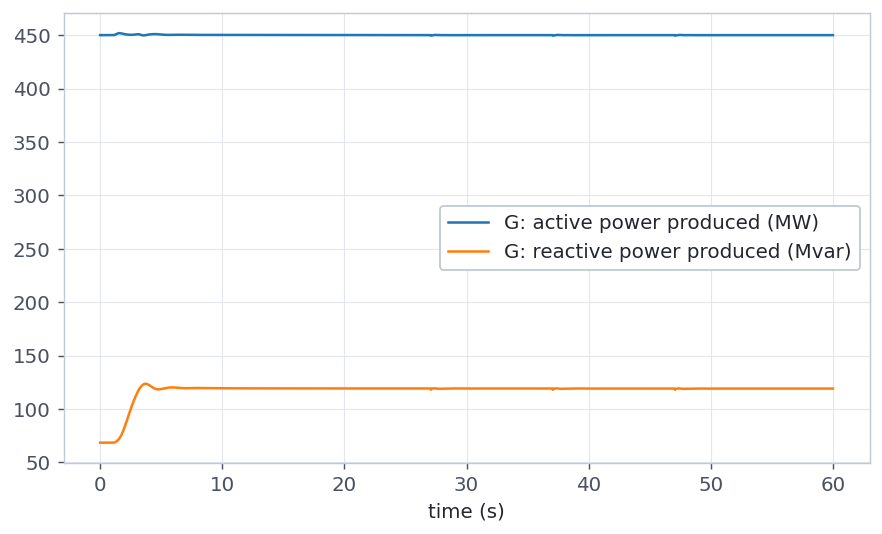
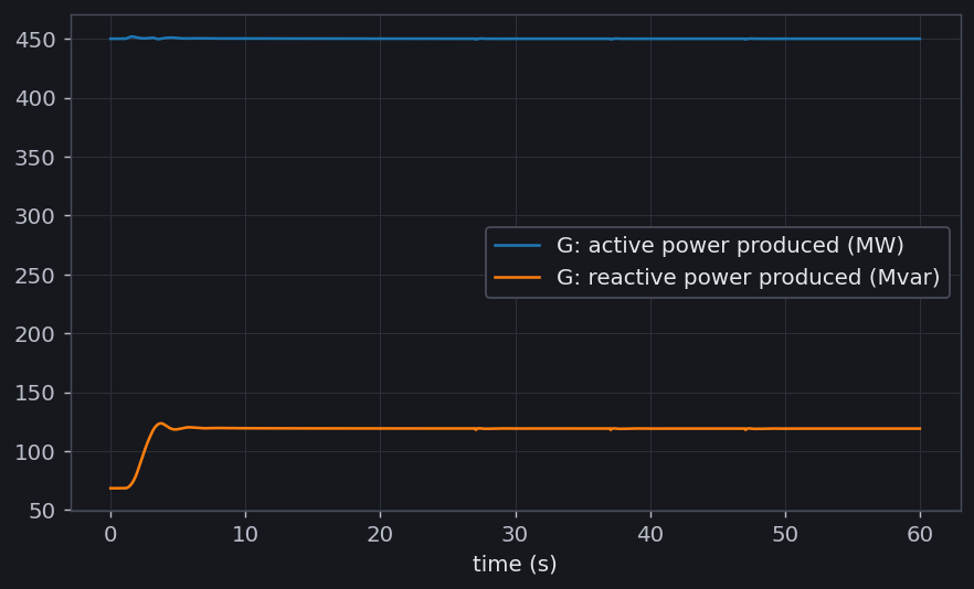
ext = stepss.extractor(case.getTrj())
ext.getSync('G').P.plot()
ext.getSync('G').Q.plot()

The exciter set point rises by 0.05 pu, so the machine’s reactive output is what moves: active power holds at its scheduled 450 MW while reactive power climbs from 68 to about 120 Mvar in a couple of seconds and settles there.