Integrator Blocks

Integrators with a time constant, optionally bounded by fixed or variable non-windup limits.

---

int

Integrator with (positive) time constant $T$.

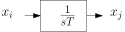
Syntax

& int
x_i
x_j
{T}

x_i is the input, x_j is the integrated output, and T is the (positive) time constant (data name, parameter name, or math expression).

Internal states: none

Discrete variables: none

Equation

$T\,\dot{x}_j = x_i$

Notes

$T = 0$ is not allowed. If $T$ is too small, the solver may encounter a singularity and the simulation may fail.

---

inlim

Integrator with (positive) time constant $T$ and non-windup limits on output.

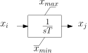
Syntax

& inlim
x_i
x_j
{T}
{x_min}
{x_max}

x_i is the input, x_j is the limited integrated output. T is the time constant; x_min and x_max are constant output limits (data names, parameter names, or math expressions).

Internal states: none

Discrete variable: $z \in \{0, 1, -1\}$

Equations

$$\begin{aligned} T\,\dot{x}_j &= x_i && \text{if } z = 0 \\ 0 &= x_j - x_{min} && \text{if } z = -1 \\ 0 &= x_j - x_{max} && \text{if } z = 1 \end{aligned}$$

Discrete transitions

if z = 0:
    if x_j > x_max:
        z ← 1
    else if x_j < x_min:
        z ← -1
else if z = 1:
    if x_i < 0:
        z ← 0
else:  # z = -1
    if x_i > 0:
        z ← 0

Initialization

if x_j > x_max:
    z ← 1
else if x_j < x_min:
    z ← -1
else:
    z ← 0

Notes

The limits are non-windup: when the output reaches a limit, integration stops and the limit is enforced as an algebraic constraint. Integration resumes (in the direction away from the limit) once the input drives the output back into the feasible range.

$T = 0$ is not allowed. If $T$ is too small, the solver may encounter a singularity and the simulation may fail.

---

invlim

Integrator with (positive) time constant $T$ and non-windup limits on output. The lower and upper limits are variables.

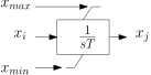
Syntax

& invlim
x_i
x_min
x_max
x_j
{T}

x_i is the input; x_min and x_max are variable (state) lower and upper limits; x_j is the limited integrated output; T is the time constant (data name, parameter name, or math expression).

Internal states: none

Discrete variable: $z \in \{0, 1, -1\}$

Equations

$$\begin{aligned} T\,\dot{x}_j &= x_i && \text{if } z = 0 \\ 0 &= x_j - x_{min} && \text{if } z = -1 \\ 0 &= x_j - x_{max} && \text{if } z = 1 \end{aligned}$$

Discrete transitions

if z = 0:
    if x_j > x_max:
        z ← 1
    else if x_j < x_min:
        z ← -1
else if z = 1:
    if x_i < 0:
        z ← 0
else:  # z = -1
    if x_i > 0:
        z ← 0

Initialization

if x_j > x_max:
    z ← 1
else if x_j < x_min:
    z ← -1
else:
    z ← 0

Notes

Unlike inlim, the bounds $x_{min}$ and $x_{max}$ are model states (variables) that can change during simulation, enabling dynamic limit adjustment.

The non-windup behaviour is identical to inlim: integration halts when a limit is reached and resumes once the input drives the output away from that limit.

$T = 0$ is not allowed. If $T$ is too small, the solver may encounter a singularity and the simulation may fail.

---

See Also

• Block Index, all CODEGEN blocks by category
• CODEGEN Model Examples, complete models built from these blocks
• User-Defined Models, the DSL file format