The Interface

The window is six tabs, and you use them roughly left to right: name the files, choose what to record, solve the initial operating point, run the simulation, then analyse the result. The sixth builds your own models.

This page says what each tab is for. It does not describe the file formats themselves; File Formats and Dynamic Data Records own those.

System Data

Where the case is named. Nine numbered rows take the system data files, and a separate row below takes the disturbance file. Both groups are required.

Each row has a Load file button and a pencil that opens the file in an editor. Clear files empties the tab.

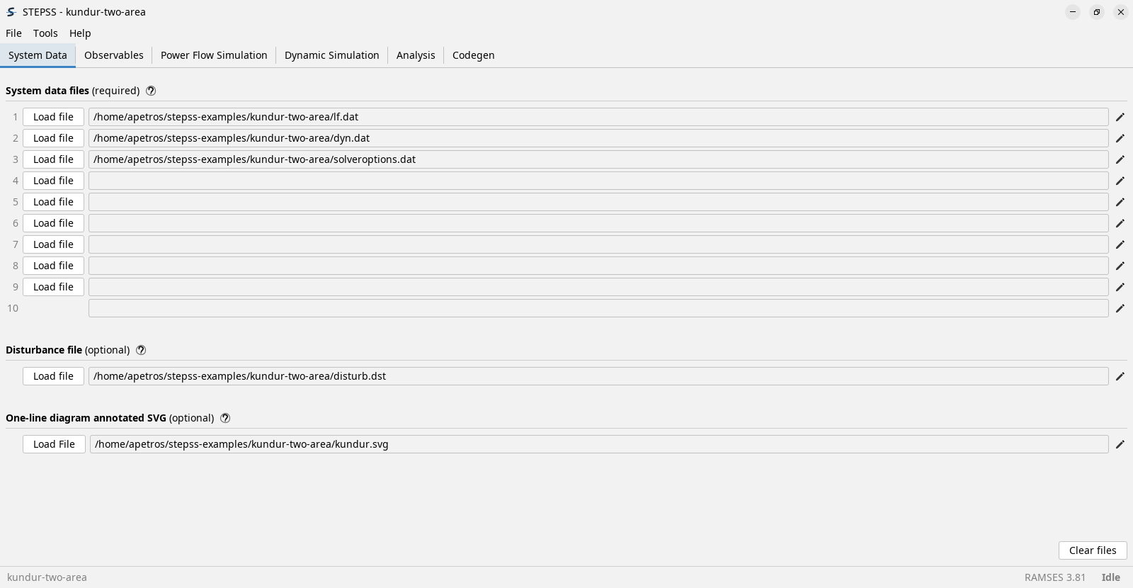
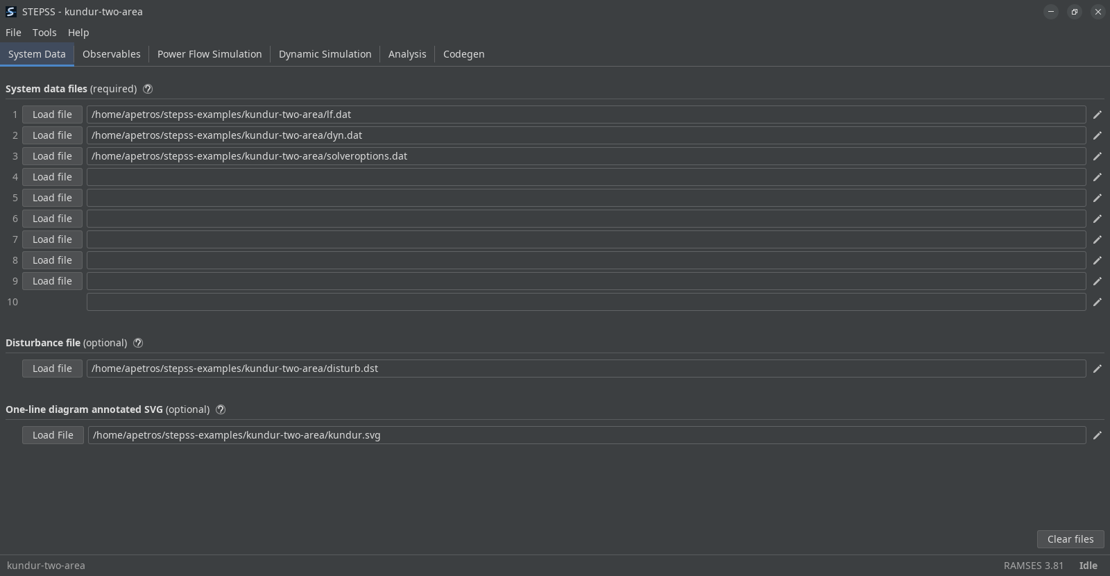
The System Data tab with the Kundur two-area case loaded. Rows one to three hold the load flow, dynamic data and solver options files; rows four to ten are empty. Below them a disturbance file row, marked optional, holds disturb.dst, and a third group, the optional one-line diagram annotated SVG, holds kundur.svg.

Order does not matter and the rows need not be filled contiguously. Which files a case needs depends on the study: a network description, dynamic component data and solver settings are the usual three.

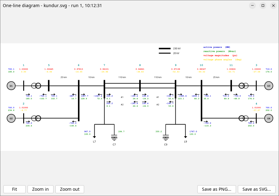
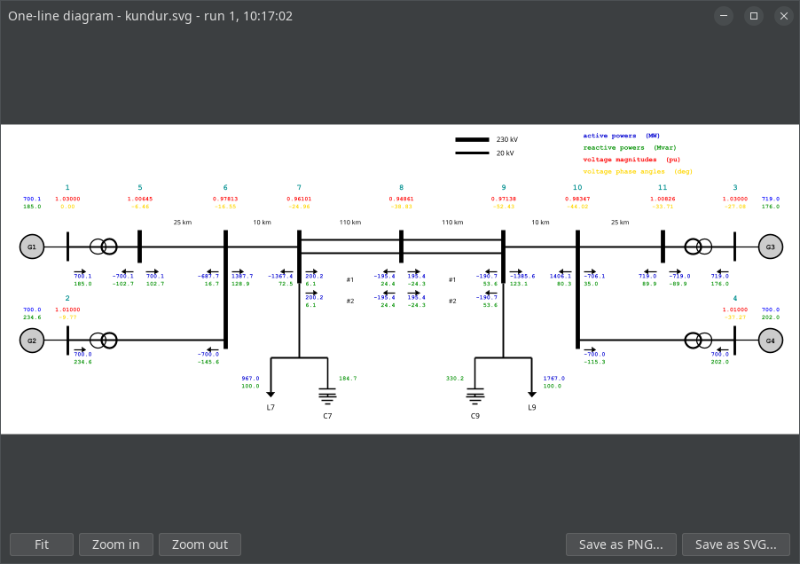
The last row takes an annotated SVG one-line diagram, a drawing of the network with placeholder codes typed into it. Every Run power flow fills those codes in with the solved values and opens the result in a window of its own; Annotated One-line Diagram owns the codes and the authoring.

Observables

Two separate jobs share this tab: what you watch while the simulation runs, and what gets written to disk for afterwards.

Runtime observables

Three rows, each pairing a quantity with the name of the equipment to watch. Fill any of them in and STEPSS plots those quantities live as the simulation advances.

The quantities on offer are bus voltage, machine speed, omega-delta and active power-delta of a machine, centre of inertia, wall time, latency, branch active and reactive power at either end, and an injector observable. The name beside it is the equipment’s own: a bus name for a bus voltage, a synchronous machine name for a speed or a centre of inertia, and RT for wall time, which plots wall clock against simulation time.

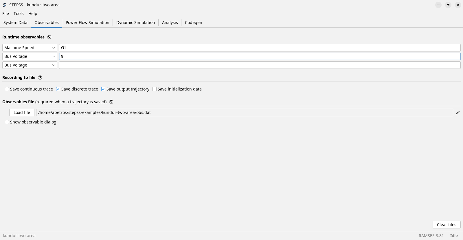
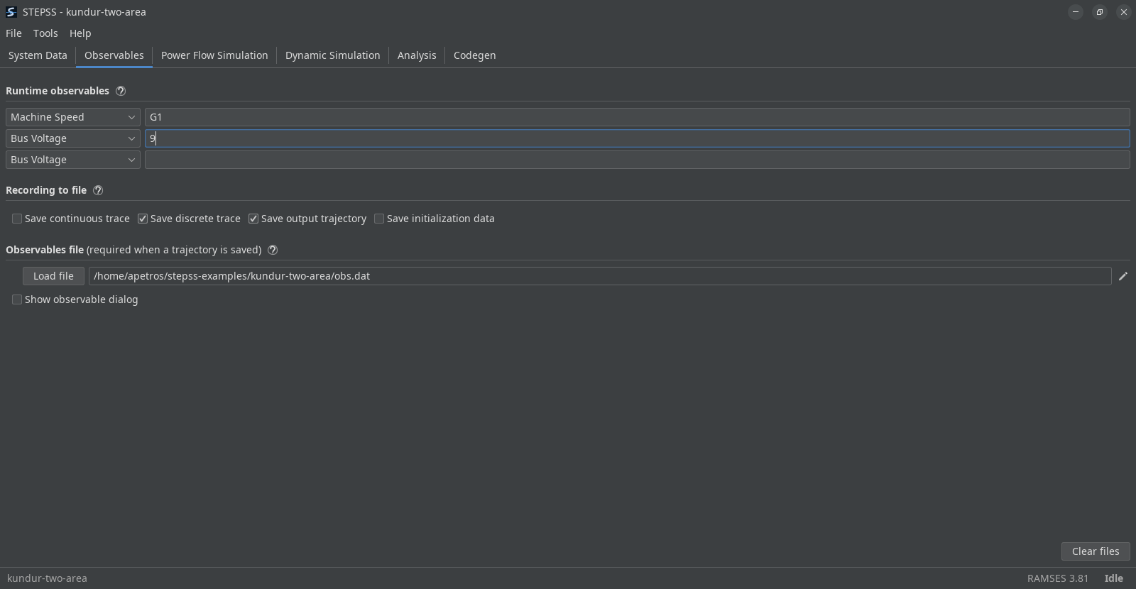
The Observables tab. Runtime observables are set to machine speed of G1 and the voltage of bus 9. Below, Save discrete trace and Save output trajectory are checked, and the observables file obs.dat is loaded.

A quantity may be followed by extra gnuplot commands, separated by /. They are passed through into the .plt script the engine writes, for anyone who opens that file in gnuplot. They have no effect on the curves STEPSS draws.

Live plotting needs nothing installed; see First Run.

Recording to file

Four independent choices, on one row: save the continuous trace, the discrete trace, the output trajectory, and the initialization data. The last of those writes the settings, the comments and the initialization data to dump.trace; hover any of the four for what it records.

The observables file below them is required whenever a trajectory is saved, because it is what says which quantities the trajectory should contain. Observables File gives its syntax and the eight equipment types it accepts. Show observable dialog builds one interactively instead of writing it by hand.

Ticking it opens eight rows under the tab, one per equipment type. Name a piece of equipment and Add puts it on that row’s list, All takes every one of that type in the case, and the list beside it is what will be recorded.

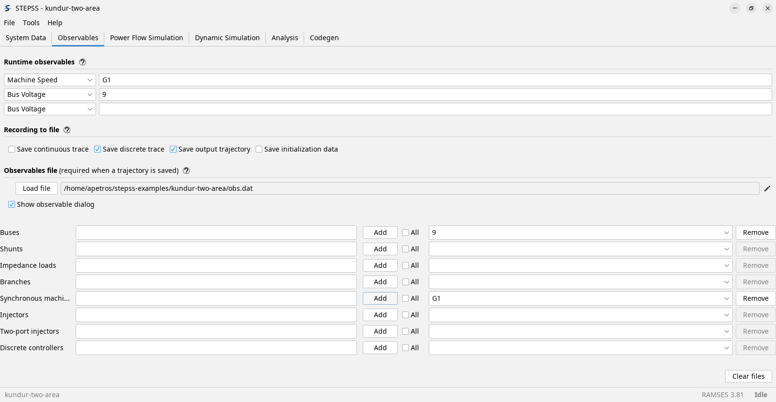
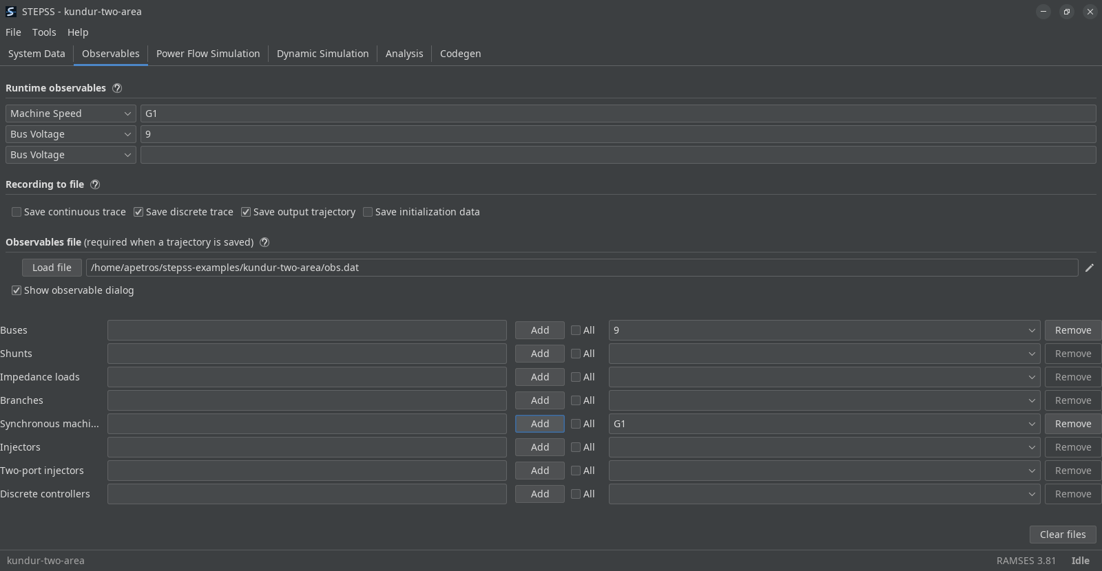
The Observables tab with Show observable dialog ticked. Eight rows appear below it, one each for buses, shunts, impedance loads, branches, synchronous machines, injectors, two-port injectors and discrete controllers. Every row has a name field, an Add button, an All tick, a drop-down of what has been chosen and a Remove button. Bus 9 has been added on the Buses row and machine G1 on the synchronous machines row.

The eight lists are session state and are not written into a saved configuration, so a case saved with the box ticked comes back needing them filled in again.

Power Flow Simulation

Where the power flow is solved, giving the operating point the dynamic simulation starts from.

Run power flow calls Helios and reports into the pane above: bus voltages and angles, the generator table with its limits, the system power balance, and the files it exported.

Seven buttons enable once a run succeeds:

Button	What it does
Add Helios results to data	Puts the solved `in_volt_trfo.dat` into system data row ten, so the dynamic simulation starts from this operating point
Save power flow solution	Keeps a copy of that file, which the next run would otherwise overwrite
Bus overview	Bus voltages and angles
Branch flows	P and Q at each end, losses, and loading against rated MVA
Generators & SVCs	Generator and SVC output, against their limits
Adjustable transformers	Transformer ratios, including any Helios adjusted
Global power balance	Generation, load, shunts and network losses

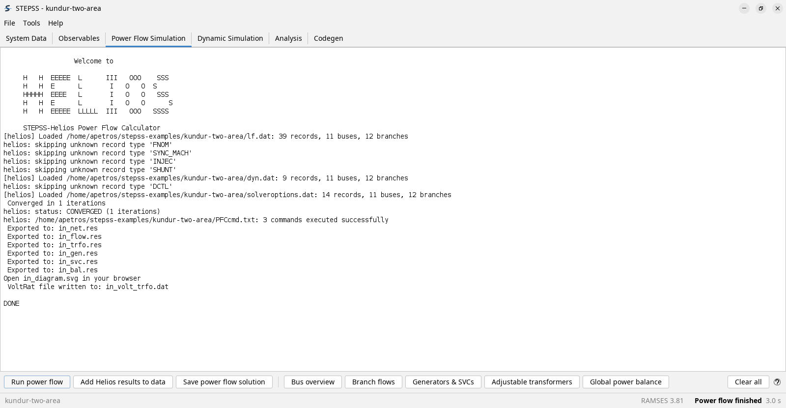
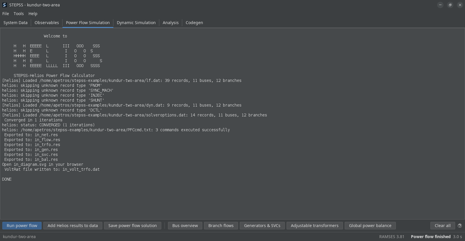
The Power Flow Simulation tab after a successful run on the Kundur case. The pane shows the Helios log: three data files loaded, status CONVERGED in one iteration, and six result files exported. The inspection buttons below, Bus overview, Branch flows, Generators and SVCs, Adjustable transformers and Global power balance, are enabled, and the status bar reads Power flow finished, 3.0 s.

Each of the four inspection buttons writes its table into the same pane, so the run’s log and the answer you asked for stay in one place.

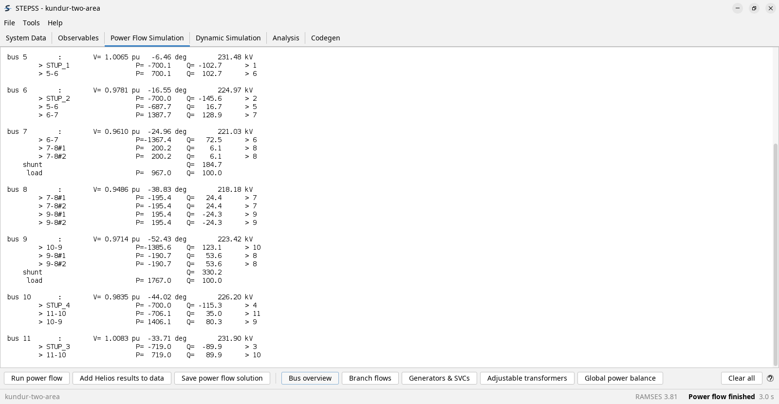
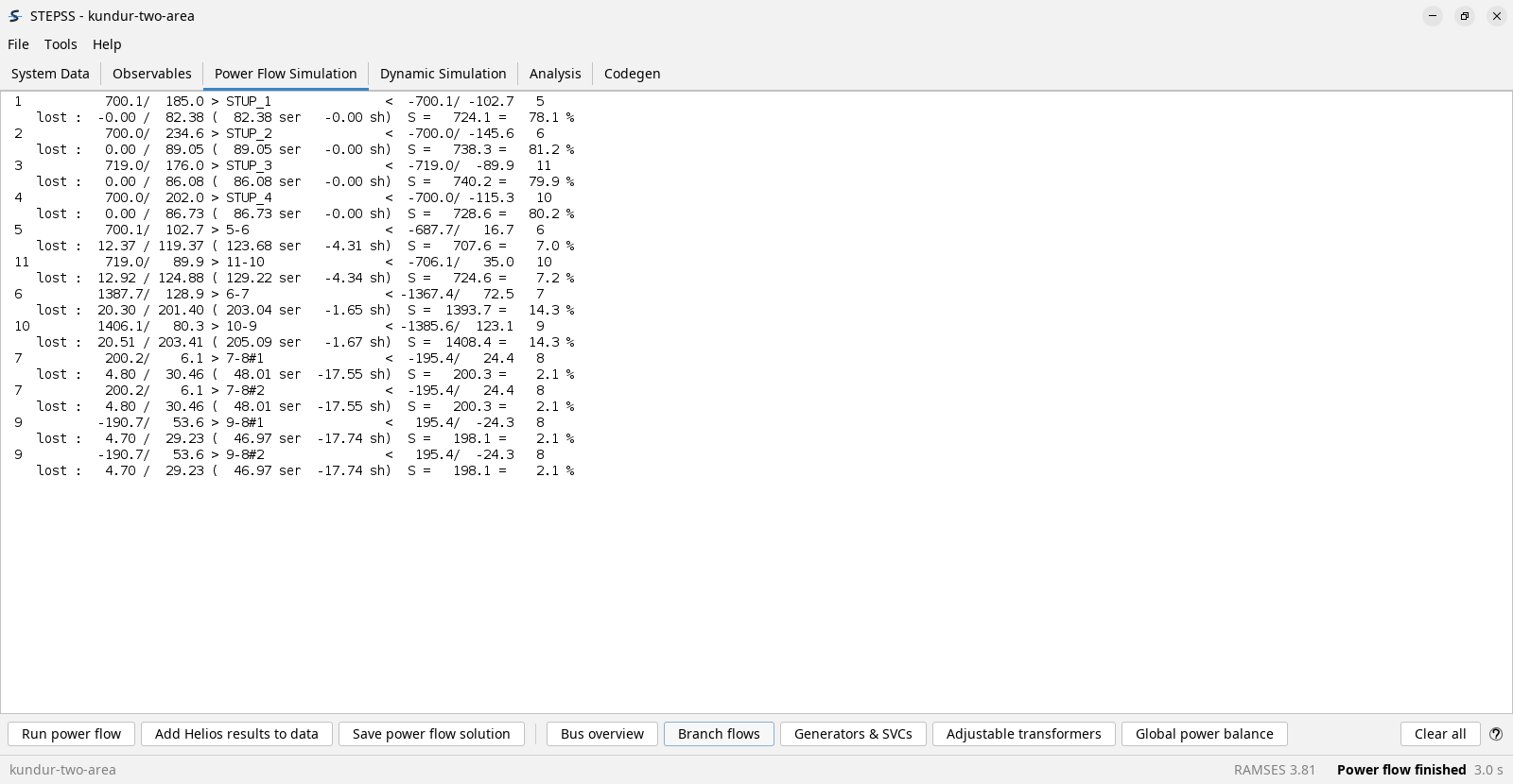
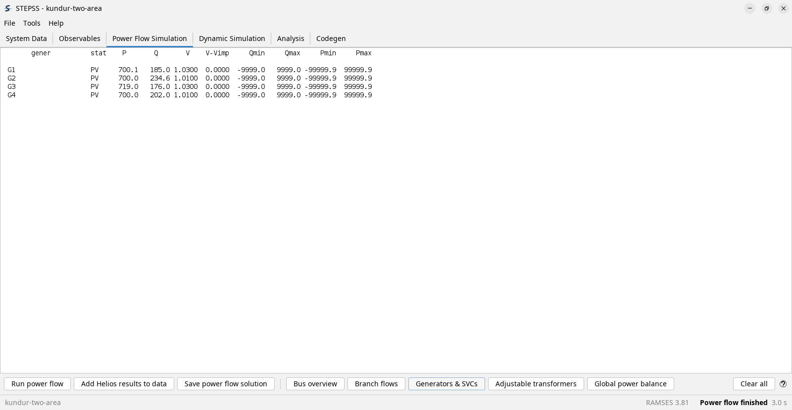
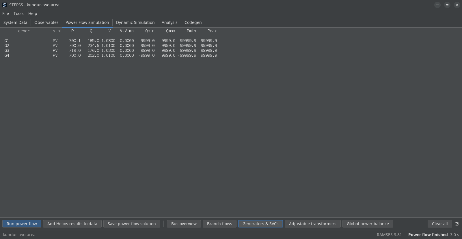
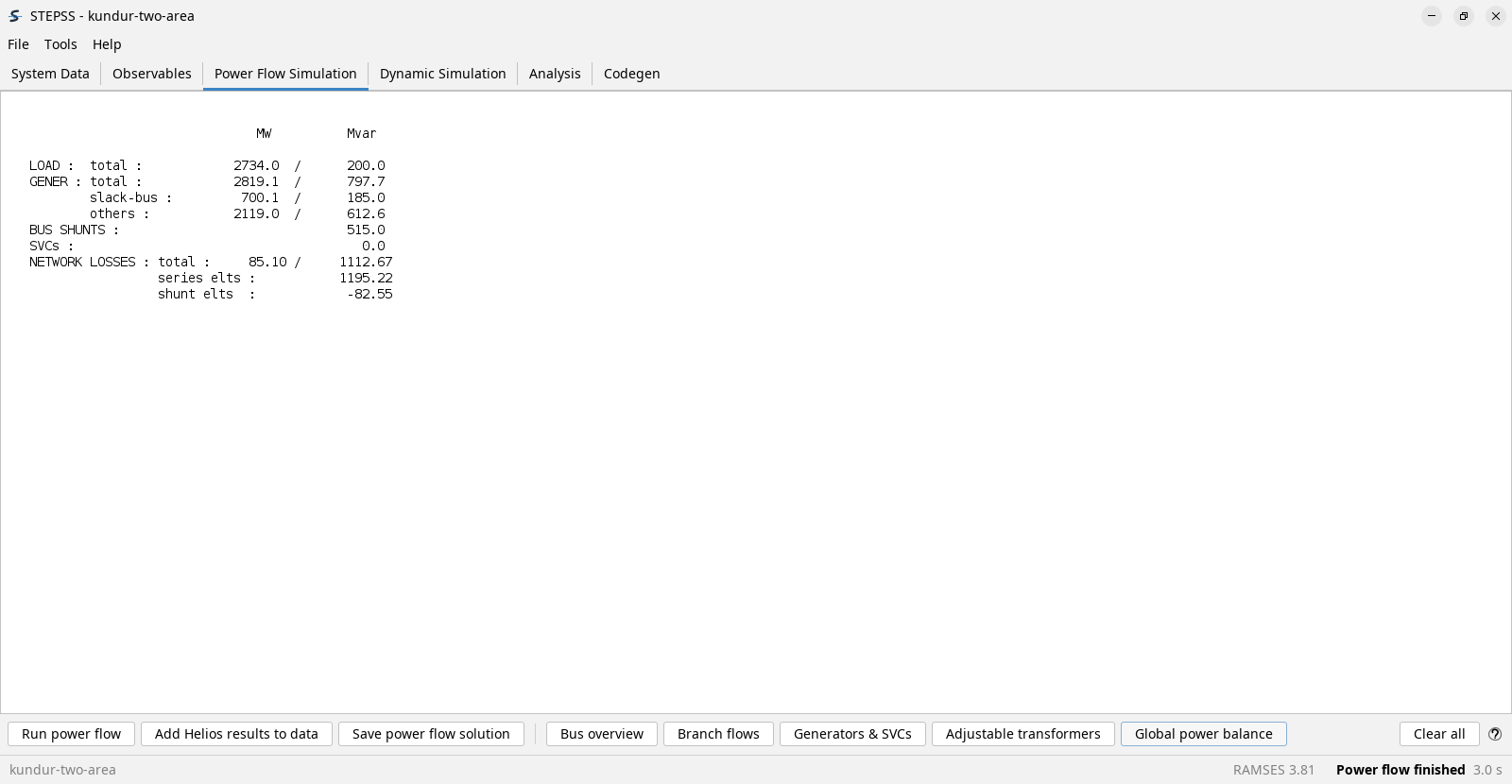
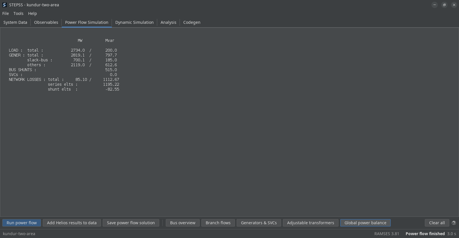
The Power Flow Simulation pane showing the bus overview for the Kundur case. Each bus is a block giving its voltage in per unit, its angle in degrees and its voltage in kilovolts, followed by one indented line per branch, shunt and load at that bus with the P and Q flowing into it and the bus at the other end.

Adjustable transformers has no tab above it because the Kundur case has no adjustable transformer to report; on a case that has them, it lists each one’s ratio and marks any that Helios moved.

A case that also loaded a one-line diagram gets a window of its own on every run, with the solved values substituted into the drawing.

The one-line diagram window for the Kundur case, titled One-line diagram, kundur.svg, run 1. The two areas are drawn with their four machines, eleven buses and the double tie between buses 7 and 9, and every placeholder in the drawing has been replaced by a solved value: active powers in blue, reactive powers in green, voltage magnitudes in red and phase angles in orange, with a key at the top right. Fit, Zoom in and Zoom out sit at the bottom left, Save as PNG and Save as SVG at the bottom right.

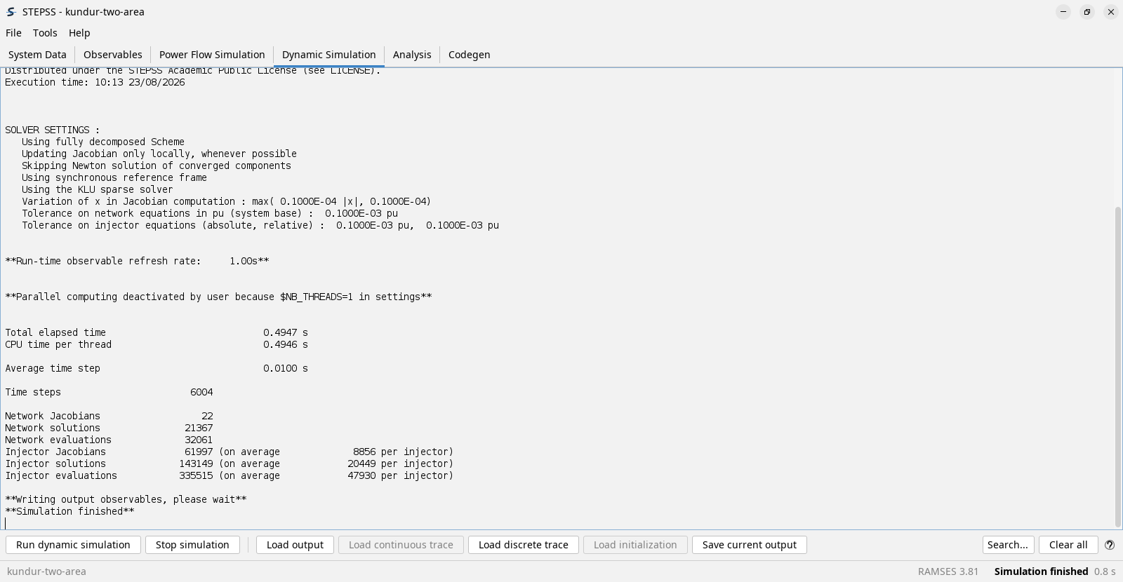
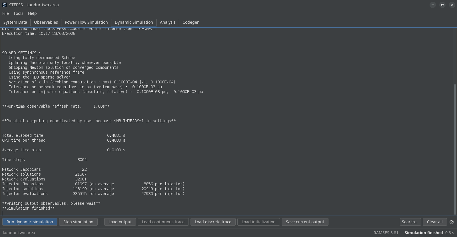
Dynamic Simulation

Where the case is run. Run dynamic simulation starts RAMSES and Stop simulation ends it early.

The pane reports the settings in force, the integration method and tolerances, whether parallelism is active, and on completion the elapsed time, the number of time steps, and Jacobian, solution and evaluation counts for the network and the injectors. Those counts are how you tell a cheap run from an expensive one.

The load buttons beside them read back a previous run’s output, continuous trace, discrete trace or initialization data, so a result can be examined without re-running it. Search finds text in the pane.

The Dynamic Simulation tab after a completed run. The pane lists the solver settings in force, the synchronous reference frame and the KLU sparse solver among them, notes that parallel computing is deactivated because the case sets one thread, then reports about half a second of elapsed time over 6004 time steps at an average step of 0.01 seconds, with Jacobian, solution and evaluation counts for the network and the injectors, ending in Simulation finished.

Analysis

Two kinds of analysis, on the same solved case.

Time-domain analysis turns a saved trajectory into curves. Extract curves opens a picker and then draws the result in a window of its own, one per extraction, so two extractions can be compared side by side. Each window saves its own figure as PNG, SVG or CSV, and its own .cur and .plt pair for plotting in gnuplot yourself. Save output trajectory writes the whole trajectory. Load trajectory reads a trajectory from an earlier run. Close all curve windows closes every curve window at once. Running a Simulation walks through this.

Small-signal stability analysis runs the engine’s eigenanalysis at a chosen instant. Point it at a results directory, set a basename and the analysis time, then Run small-signal stability analysis.

There are no thresholds here. There used to be a real-part limit and a participation factor threshold, and both decided what the engine would write; every mode is written now, and the thresholds live in the results window where changing one re-filters what is already on screen. See Eigenanalysis. Each run opens its own results window and leaves any already up alone, so two runs can be compared side by side. Save dynamic Jacobian… and Load dynamic Jacobian… write that run out as an archive and open it again later, each load in a window of its own too.

The analysis needs $SCHEME DE and $OMEGA_REF SYN, and the button supplies both: it writes them into one small data file read after your own, where being last is what makes them win. So a case set up for time-domain runs analyses as it stands, and your own solver settings are neither edited nor left changed afterwards.

Output, below both sections, is where the tools on this tab report. The engine’s small-signal run and both DYNGRAPH invocations behind Extract curves write here, so a run that produced nothing says why on the tab that started it. Save output… writes the pane to a file and Clear output empties it. Before STEPSS 3.81 the engine wrote to the Dynamic Simulation tab instead, underneath whatever an earlier time-domain run had left there, and DYNGRAPH reported nothing at all unless it failed.

This is performed by RAMSES itself. Eigenanalysis explains the method, the settings and what the results mean.

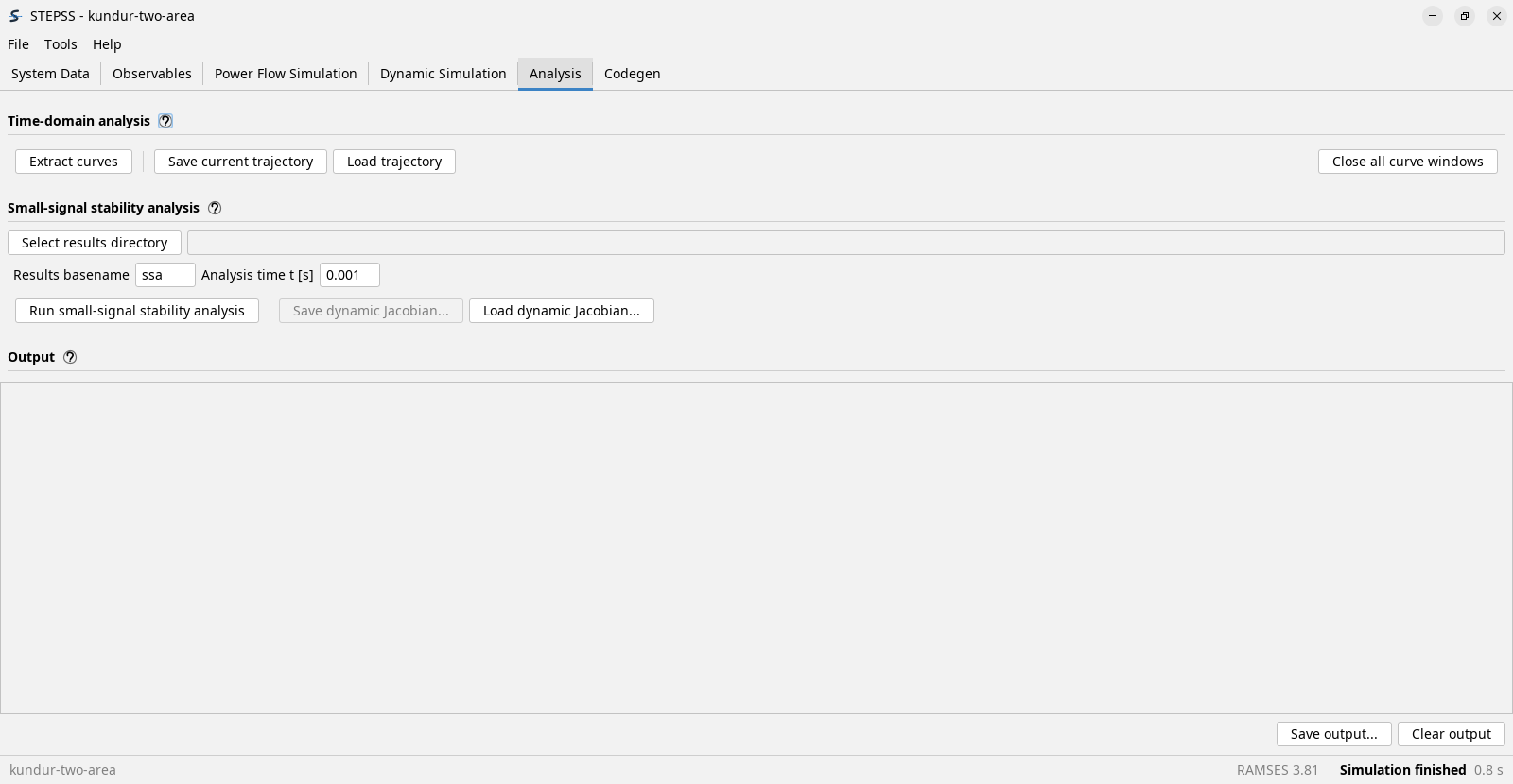
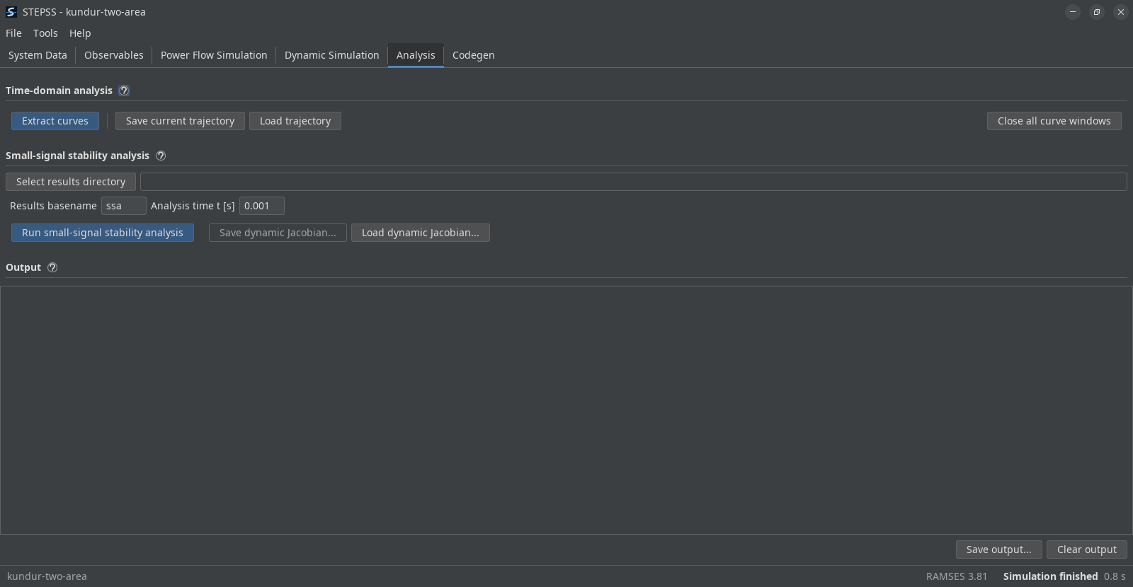
The Analysis tab with a completed run available. A Time-domain analysis row offers Extract curves, Save current trajectory and Load trajectory, with Close all curve windows at the right. Below it a Small-signal stability analysis section offers Select results directory beside an empty field, a basename of ssa and an analysis time of 0.001 seconds, with buttons to run the analysis and to save or load the dynamic Jacobian. An Output console fills the rest of the tab, with Save output and Clear output beneath it.

The unlabelled field beside Select results directory is where results are written, and it defaults to the working directory. The picker that Extract curves opens, and the small-signal results window, are both shown on the pages linked above.

Codegen

Where a model of your own becomes part of the simulator, in the order the buttons run:

Button	What it does
Load files for Codegen	Takes one or more model descriptions in the CODEGEN language
Run Codegen	Translates them into Fortran, reporting each block with its equation and state counts
Display loaded files	Lists the Fortran files generated so far, not the descriptions that were read
Save converted files	Writes the generated `.f90` out
Compile	Builds and links it against the engine, giving a custom simulator
Save executable	Keeps that simulator, rather than rebuilding it next time

Each enables as the previous step makes it meaningful. Once a custom simulator exists, simulations run on it rather than on the bundled engine.

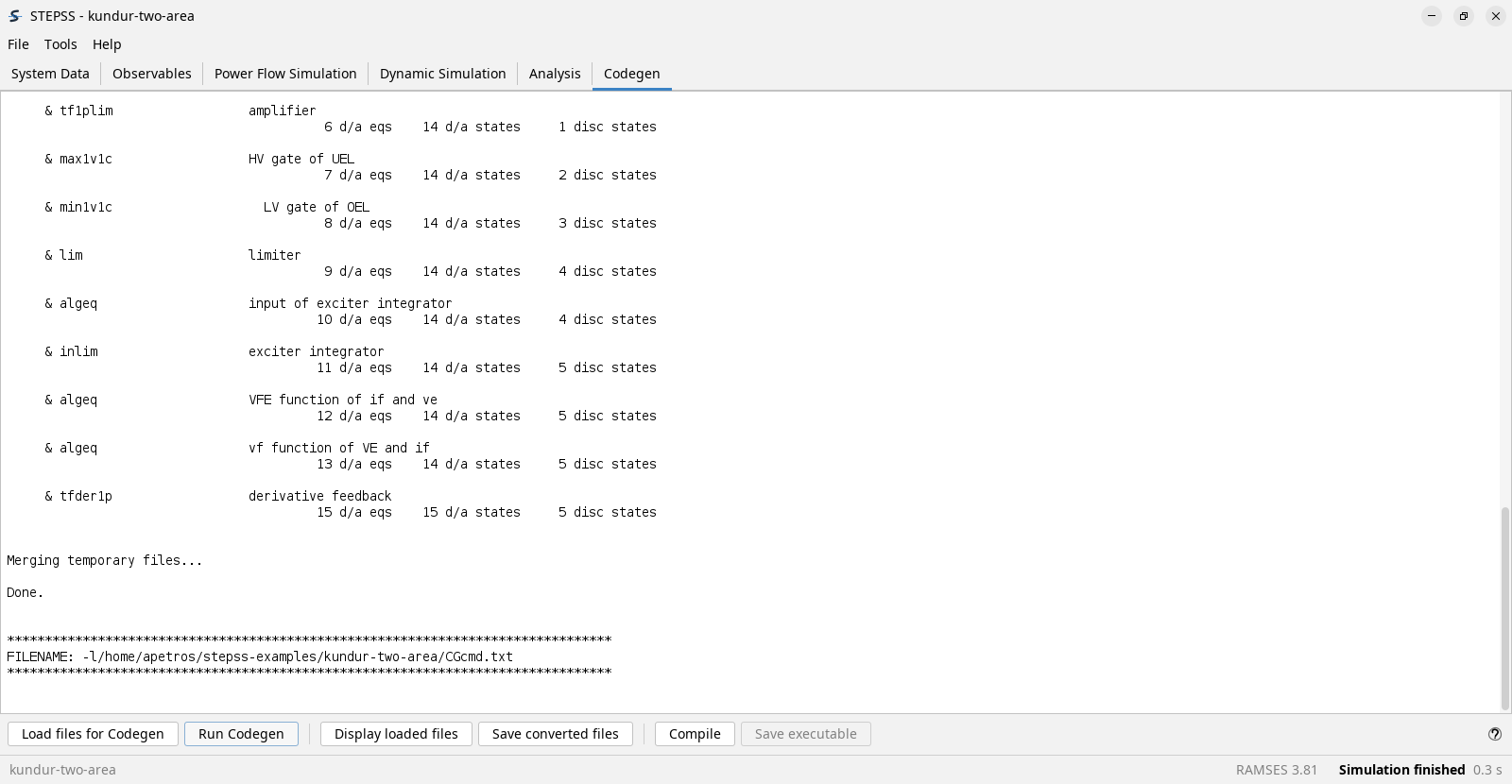
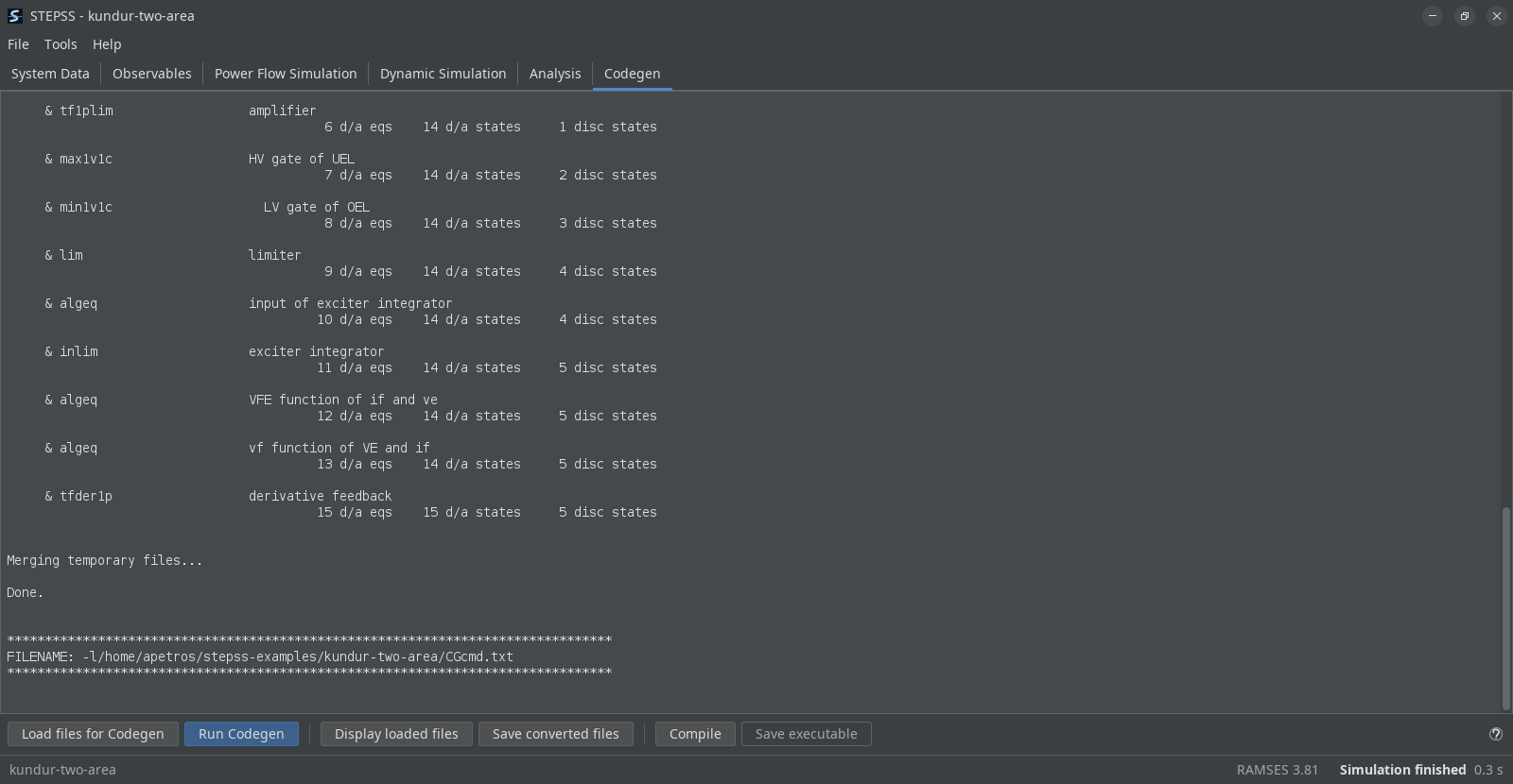
The Codegen tab after running CODEGEN on an IEEE AC1A exciter description. The pane logs each translated block in turn, an LV gate, a limiter, algebraic equations, the exciter integrator and a derivative feedback, each with its running count of differential-algebraic equations, states and discrete states, then reports merging the temporary files and Done. Save converted files and Compile are now enabled.

Compiling needs a Fortran toolchain on the machine, which is its own installation step; translating a model does not.

User-Defined Models is the reference for the model language, and CODEGEN Studio assembles models visually instead of by hand.

The menus

File holds Save configuration and Load configuration, plus Open Examples and Exit.

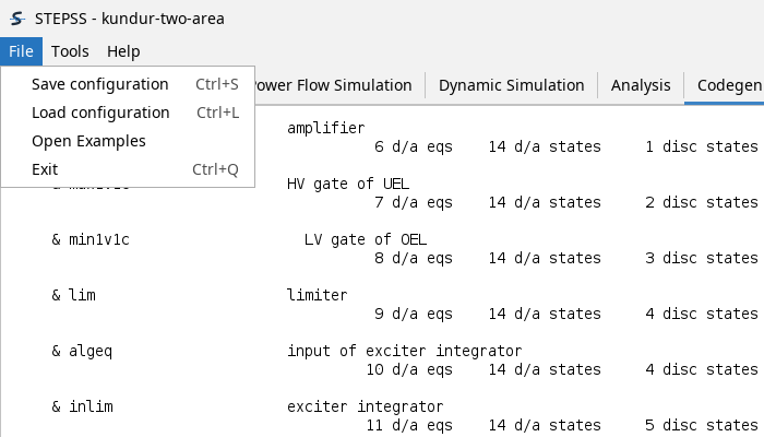
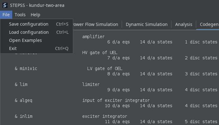
The File menu open, holding Save configuration with Ctrl+S, Load configuration with Ctrl+L, Open Examples, and Exit with Ctrl+Q.

Save configuration writes a .cfg holding everything a run is made of: the ten system data rows, the disturbance and observables files, the three runtime observable rows, and the four recording checkboxes. Load configuration puts them back, so a case set up once can be reopened and run in two clicks. A path inside the .cfg’s own folder is stored relative to it, which means the folder can be moved, copied or sent to a colleague whole; anything outside that folder is stored as an absolute path and stays tied to the machine that saved it.

The file is plain text and documented key by key in Scenario File, so one can be written by hand or generated by a script.

Two things the file does not carry. The observable dialog’s five picker lists are not saved, so a configuration saved with Show observable dialog ticked says so when it loads and the lists need filling in again. And .cfg files written by STEPSS releases before this format are refused rather than loaded: they hold absolute paths belonging to whoever last saved them, so what they name almost never exists on the machine opening them. Set the case up and save it again.

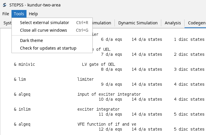
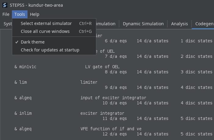
Tools holds Select external simulator and Close all curve windows; and, below a separator, the Dark theme toggle and Check for updates at startup. The last two are ticks rather than actions, and both are remembered between sessions.

The Tools menu open, holding Select external simulator with Ctrl+R and Close all curve windows with Ctrl+G, then below a separator the Dark theme and Check for updates at startup ticks, both unticked.

The Tools menu open, holding Select external simulator with Ctrl+R and Close all curve windows with Ctrl+G, then below a separator the Dark theme tick, which is ticked, and Check for updates at startup.

A case is saved and reopened through File > Save configuration, which writes the scenario file. Quick Start compares the two ways to drive the engines.

The status bar

The working directory on the left; on the right the engine version and what the application is doing. That last field runs from Idle through Solving power flow to Power flow finished and Simulation finished, each with the elapsed time, which is the quickest confirmation that a run actually did something.