

First Run
STEPSS GUI is the desktop edition: the one an installer puts on your machine, and the one that carries every engine plus CODEGEN. This page covers the first launch and gets you to a working simulation without you supplying any data of your own.
If it is not installed yet, start at Installing STEPSS GUI.
Accepting the licence
Section titled “Accepting the licence”The first launch shows a licence and will not continue until you accept it.
The licence on that screen is RAMSES’s, not the interface’s. The two user interfaces are Apache 2.0, while the dynamic simulator is the property of the University of Liège and free for non-commercial use only, so the dialog names the component rather than the application. The free version is also capped, in ways worth knowing before you build a large case.
License is the one page that states the terms, the caps and which component each applies to. Read it there rather than inferring them from the dialog.
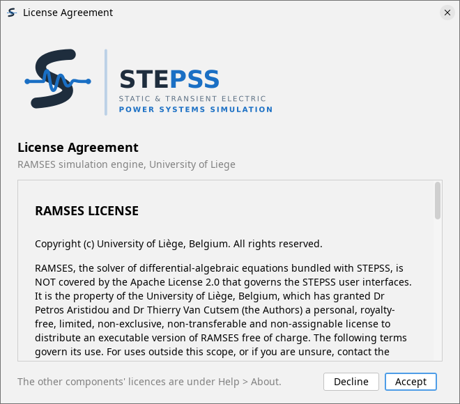
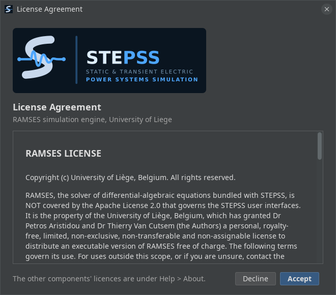
You accept once. Later launches go straight to the window.
Start from a bundled example
Section titled “Start from a bundled example”The fastest way to see STEPSS work is not to load anything of your own. The application ships four complete test systems, and opening one copies it to disk and fills in every file slot, so Run works immediately.
-
Open the File menu.
-
Choose Open Examples.
-
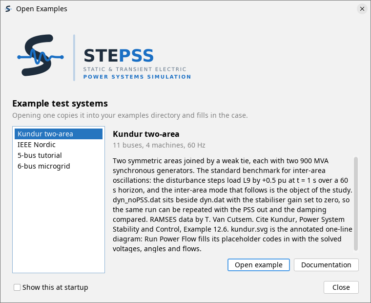
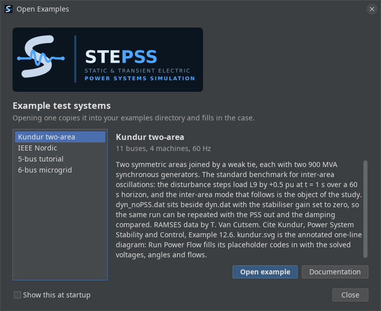
Pick a system from the list. The panel beside it describes the case, its size and what the shipped disturbance does.
-
Click Open example.
-
Answer Choose a directory to keep examples in. This is asked once per session rather than once ever, because the choice is not remembered between launches. Any directory you can write to will do, and the same one every time keeps your cases together.
A banner across the top of the window then reports where the copy landed, with an Open folder button to reveal it, and Dismiss to put it away. Behind it every file slot is already filled in.
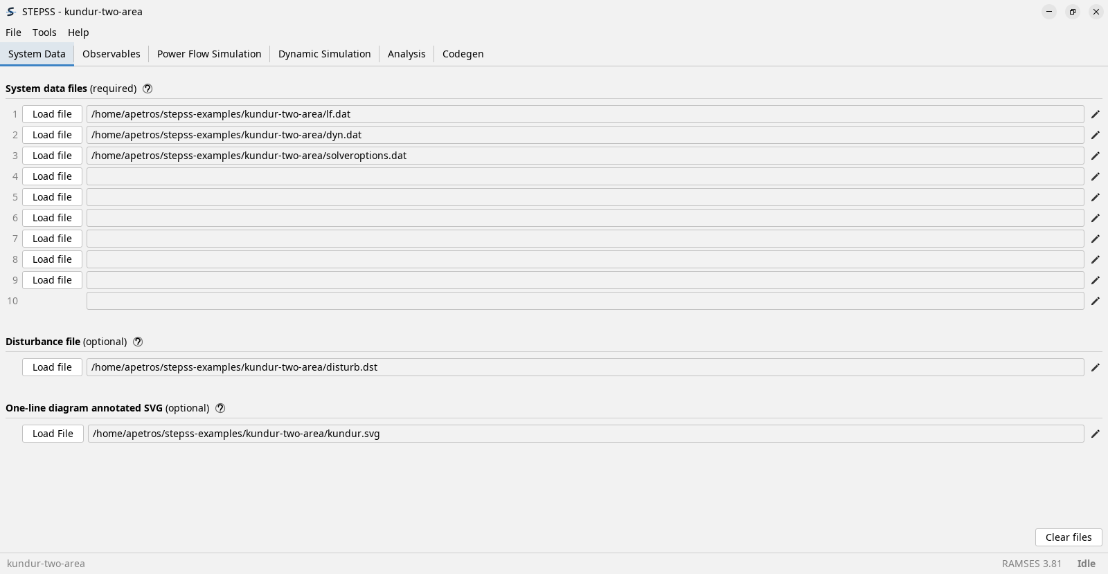
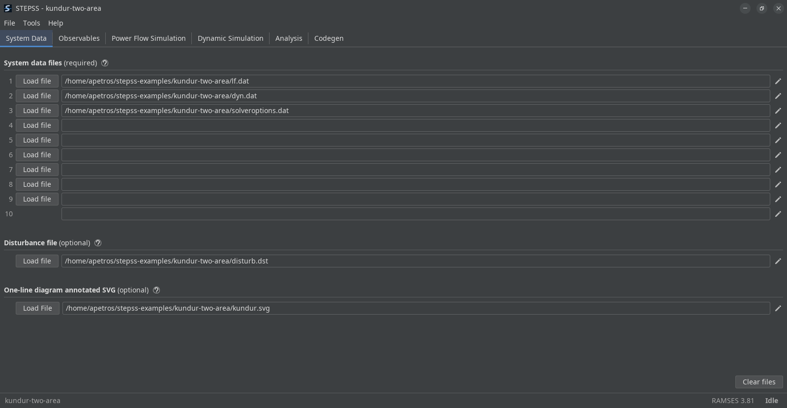
The dialog appears on startup by default. Clear Show this at startup to stop that, and reach it from File, Open Examples whenever you want it back.
The four bundled systems
Section titled “The four bundled systems”| System | Size | What it is for |
|---|---|---|
| 5-bus tutorial | 5 buses, 1 machine | The teaching case from EEN452 at the Cyprus University of Technology, and the one to open first. One generator with detailed machine, governor and AVR models, a composite load, and an external grid, small enough to read end to end. Its disturbance file is deliberately empty, ready for you to add the records of the study you want. |
| Kundur two-area | 11 buses, 4 machines, 60 Hz | The standard benchmark for inter-area oscillations. Two symmetric areas joined by a weak tie. The shipped disturbance steps a load and the resulting inter-area mode is the object of the study. A second dynamic file with the stabiliser disabled ships beside the first, so the same run can be repeated with the PSS out and the damping compared. |
| IEEE Nordic | 74 buses, 20 machines, 400/220/130 kV | The reference system for long-term voltage stability, from IEEE PES technical report PES-TR19. It opens on the tripped-branch case it is best known for, with further disturbances, a second operating point and a set of load-increase variants shipped alongside. |
| 6-bus microgrid | 6 buses, 2 generators, 6/11 kV | A power-flow-only case: two lines, four transformers, loads at buses D and E, and generators at A (slack) and F. It carries no dynamic data and no disturbance scenario, so it runs on Power Flow Simulation and not on Dynamic Simulation. It is the case the annotated one-line diagram is demonstrated with: 6bus.svg is a template of placeholder codes that Run power flow fills in with the solved values. |
The first three link to their own page here, which carries the network, the models and the studies the system is used for. The microgrid has no page of its own, because everything it demonstrates belongs to Power Flow, so its name links to its repository instead. Documentation in the dialog opens the system’s source repository in every case.
Where the files go
Section titled “Where the files go”Two directories are kept separately, and the distinction matters once you open more than one example.
- The examples directory is where copies are unpacked. You are asked for it the first time you open an example, and it is kept for as long as the application stays open. Opening a second example puts it beside the first rather than inside it.
- The working directory is where a run reads and writes. Opening an example moves it into that example.
Neither survives quitting, and neither is set from a menu: opening an example is what chooses them. The banner that reports where the copy landed has an Open folder button for getting at the files directly.
An example is copied rather than run in place, so editing it is safe and the copy survives quitting. That is the point of copying: work on it freely.
Real-time plotting
Section titled “Real-time plotting”STEPSS GUI plots curves while a simulation runs, which is covered on The Interface. It draws them itself: nothing has to be installed on any platform, and no external plotting program is involved.
Each runtime observable you filled in gets a panel of its own, stacked on a shared time axis, and the window keeps drawing until the run ends. Save PNG and Save CSV keep the picture or the samples behind it, and Reset zoom returns to the full horizon after a drag.
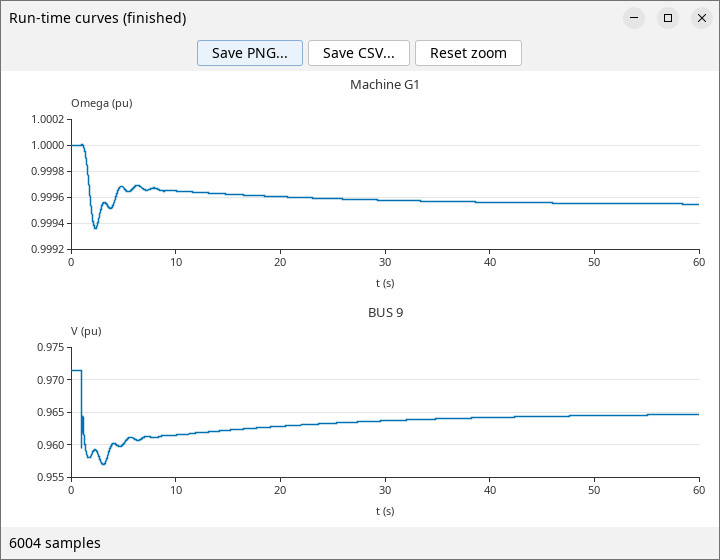
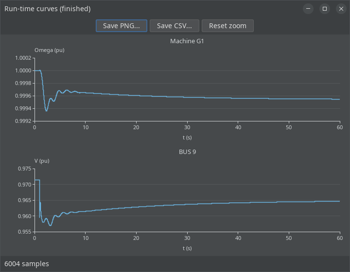
Run-time curves need a RAMSES release that writes a column map into the header of its observable file. Against an engine that does not, the window says so rather than drawing. Extracting curves after a run is independent of this: that path reads DYNGRAPH’s output, which carries no header.
Choosing a theme
Section titled “Choosing a theme”Tools, then Dark theme. The choice is remembered between sessions, along with the window’s size and position.
Next steps
Section titled “Next steps”- The Interface, what each tab is for
- Running a Simulation, a complete run on the Kundur case
- File Formats, what goes in the files you loaded