Injector Models

RAMSES custom injector models represent loads, induction machines, inverter-based resources (IBR), and battery energy storage systems (BESS) connected to network buses.

Usage in Dynamic Data Files

Injector models are defined with the INJEC keyword as standalone records in the dynamic data file. The syntax is:

INJEC model_name inj_name bus FP FQ P Q param1 param2 ... ;

Where model_name is the model identifier, inj_name is a unique instance name, bus is the connection bus, FP/FQ are participation factors, and P/Q are initial values in MW/Mvar (one of each pair must be zero, either the fraction or the absolute power).

Recognised injector model names (case-sensitive):

• Uppercase short names (no prefix): LOAD, RESTLD, THEVEQ, INDMACH1, INDMACH2, SVC_GENERIC1.
• Prefixed names: RAMSES adds the inj_ prefix automatically: VFAULT/inj_VFAULT, vfd_load/inj_vfd_load, PQ/inj_PQ, IBG/inj_IBG, WT3/inj_WT3, WT4/inj_WT4, BESS/inj_BESS, GFOL/inj_GFOL, GFOR/inj_GFOR, PMU/inj_PMU.

All of the above are built into every RAMSES distribution (standalone executable and shared library used by stepss). INDM1 and PV, documented below, have been callable since 3.79; before that they were compiled under no name. inj_norton is excluded from the build entirely and is not available: it calls a Python bridge (initialize_model_instance, call_python_evaluate) that is not part of this source tree.

Note on case sensitivity. Match the case used above exactly. The uppercase short names must be uppercase. For the prefixed family, vfd_load and VFAULT use those exact cases. Most others follow the convention inj_<UPPERCASE> (e.g. inj_PQ, inj_GFOR).

---

Load Models

LOAD (inj_load): Exponential Recovery Load

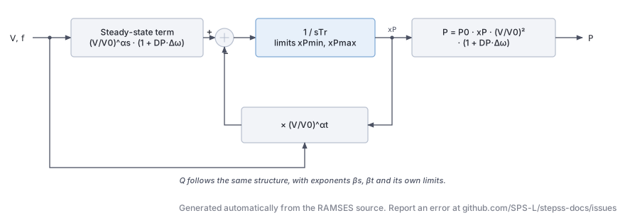
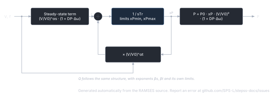
Description

The exponential recovery load model captures the transient and steady-state voltage and frequency dependency of aggregated loads. Immediately after a voltage disturbance, the load behaves according to a transient voltage exponent; it then recovers exponentially to a steady-state behaviour described by a different exponent. The model supports separate active ($P$) and reactive ($Q$) power recovery dynamics, each with individual minimum/maximum limiters on the recovery variable.

Scientific Description

The model is parameterized in terms of initial active and reactive conductance/susceptance, $G_0 = P_0/V_0^2$ and $B_0 = -Q_0/V_0^2$. Two recovery state variables $x_P$ and $x_Q$ evolve according to:

$\dot{x}_P = \frac{1}{T_r}\left[\left(\frac{V}{V_0}\right)^{\alpha_s} \left(1 + D_P\,\Delta\omega\right) - x_P \left(\frac{V}{V_0}\right)^{\alpha_t}\right]$

$\dot{x}_Q = \frac{1}{T_r}\left[\left(\frac{V}{V_0}\right)^{\beta_s} \left(1 + D_Q\,\Delta\omega\right) - x_Q \left(\frac{V}{V_0}\right)^{\beta_t}\right]$

where $\Delta\omega = \omega_{\mathrm{COI}} - 1$ is the per-unit speed deviation, $V$ is the bus voltage magnitude, $V_0$ is the initial voltage, $\alpha_t, \beta_t$ are transient exponents, $\alpha_s, \beta_s$ are steady-state exponents, and $T_r$ is the load recovery time constant. The injected currents are then:

$i_x = G_0\, x_P\, v_x\left(1 + D_P\,\Delta\omega\right) - B_0\, x_Q\, v_y\left(1 + D_Q\,\Delta\omega\right)$

$i_y = G_0\, x_P\, v_y\left(1 + D_P\,\Delta\omega\right) + B_0\, x_Q\, v_x\left(1 + D_Q\,\Delta\omega\right)$

When the recovery variable hits its limit (due to e.g. Stalling or complete voltage collapse), the limit is held until the direction of the derivative reverses.

Parameters

#	Name	Description	Unit
1	DP	Frequency sensitivity of active power	pu/pu
2	A1	Proportion of type-1 component in $P$
3	alpha1	Transient voltage exponent for $P$ (type 1)
4	A2	Proportion of type-2 component in $P$
5	alpha2	Transient voltage exponent for $P$ (type 2)
6	alpha3	Transient voltage exponent for $P$ (type 3, proportion $= 1-A_1-A_2$)
7	DQ	Frequency sensitivity of reactive power	pu/pu
8	B1	Proportion of type-1 component in $Q$
9	beta1	Transient voltage exponent for $Q$ (type 1)
10	B2	Proportion of type-2 component in $Q$
11	beta2	Transient voltage exponent for $Q$ (type 2)
12	beta3	Transient voltage exponent for $Q$ (type 3)

Internal computed parameters include the steady-state exponents for each component (derived from the transient exponents), initial conductance $G_0$, susceptance $B_0$, and initial voltage $V_0$.

State Variables

Variable	Description
iy	$y$-component of injected current (pu on system base)
ix	$x$-component of injected current (pu on system base)
xp	Active power recovery variable (dimensionless)
xq	Reactive power recovery variable (dimensionless)

Observables: P, Q, xp, xq

Usage Example

INJEC  LOAD  LOAD1  BUS1  1.  1.  0.  0.  1.5  0.3  1.0  0.2  2.0  0.5  1.8  0.4  2.5  0.1  3.0  2.0  ;

Parameters: DP A1 alpha1 A2 alpha2 alpha3 DQ B1 beta1 B2 beta2 beta3

---

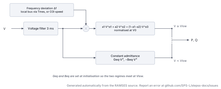
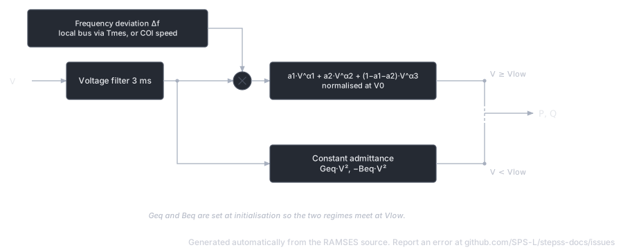
vfd_load (inj_vfd_load): Variable Frequency Drive Load

Description

The VFD load model represents aggregate industrial loads driven by variable-frequency drives, where the power consumption exhibits a composite voltage-dependent characteristic with multiple exponential components and frequency sensitivity. It also includes low-voltage protection: below a configurable threshold $V_{\min}$, the load switches to a constant-admittance representation, preventing numerical difficulties during deep voltage sags.

Scientific Description

The active and reactive powers depend on bus voltage $V$ and frequency deviation $\Delta f = f/f_0 - 1$:

$P = \left(1 + D_P\,\Delta f\right) P_0 \cdot \frac{a_1 V^{\alpha_1} + a_2 V^{\alpha_2} + (1-a_1-a_2)\, V^{\alpha_3}}{a_1 V_0^{\alpha_1} + a_2 V_0^{\alpha_2} + (1-a_1-a_2)\, V_0^{\alpha_3}}$

$Q = \left(1 + D_Q\,\Delta f\right) Q_0 \cdot \frac{b_1 V^{\beta_1} + b_2 V^{\beta_2} + (1-b_1-b_2)\, V^{\beta_3}}{b_1 V_0^{\beta_1} + b_2 V_0^{\beta_2} + (1-b_1-b_2)\, V_0^{\beta_3}}$

Below $V_{\min}$, an equivalent constant admittance is used:

$P_{\mathrm{low}} = G_{\mathrm{eq}}\, V^2, \qquad Q_{\mathrm{low}} = -B_{\mathrm{eq}}\, V^2$

where $G_{\mathrm{eq}}$ and $B_{\mathrm{eq}}$ are computed at initialization to ensure continuity at $V = V_{\min}$. The switch between the two regimes is governed by a piecewise-linear function of $V$:

$u = \begin{cases} 0 & V < V_{\min} \\ 1 & V \geq V_{\min} \end{cases}$

A small voltage filter (time constant 0.003 s) smooths the transition. The frequency deviation can optionally be computed from the local bus frequency (measured via an f_inj block with time constant $T_{\mathrm{mes}}$) or from the system centre-of-inertia speed.

The initial voltage $V_0$ can differ from the transmission bus voltage if a distribution transformer ratio is implied (set $V_{\mathrm{init}} \ne 0$ to specify the distribution-side voltage; otherwise the transmission voltage is used directly).

Parameters

#	Name	Description	Unit
1	Dp	Frequency sensitivity of active power	pu/pu
2	a1	Fraction of type-1 component in $P$
3	alpha1	Voltage exponent of type-1 $P$ component
4	a2	Fraction of type-2 component in $P$
5	alpha2	Voltage exponent of type-2 $P$ component
6	alpha3	Voltage exponent of type-3 $P$ component (fraction $= 1-a_1-a_2$)
7	Dq	Frequency sensitivity of reactive power	pu/pu
8	b1	Fraction of type-1 component in $Q$
9	beta1	Voltage exponent of type-1 $Q$ component
10	b2	Fraction of type-2 component in $Q$
11	beta2	Voltage exponent of type-2 $Q$ component
12	beta3	Voltage exponent of type-3 $Q$ component
13	Vinit	Initial distribution-bus voltage (0 = use transmission voltage)	pu
14	Vlow	Voltage threshold for constant-admittance regime (recommended 0.5–0.7)	pu
15	foption	1 = use local bus frequency; 0 = use COI speed	flag
16	Tmes	Frequency measurement time constant	s

State Variables

Variable	Description
Vreal	Voltage at equivalent distribution bus
V	Filtered distribution-bus voltage (3 ms filter)
P	Active power consumed
Q	Reactive power consumed
fbus	Local bus frequency (used if foption=1)
df	Frequency deviation $\Delta f$
u	Regime switch (1 = above $V_{\min}$, 0 = constant admittance)

Observables: P, Q, df, u

Usage Example

INJEC  vfd_load  VFD1  BUS_IND  1.  1.  0.  0.  1.5  0.7  2.0  0.2  1.0  0.5
                                 1.2  0.5  2.5  0.1  1.5  0.8
                                 0.0  0.6  0  0.1  ;

---

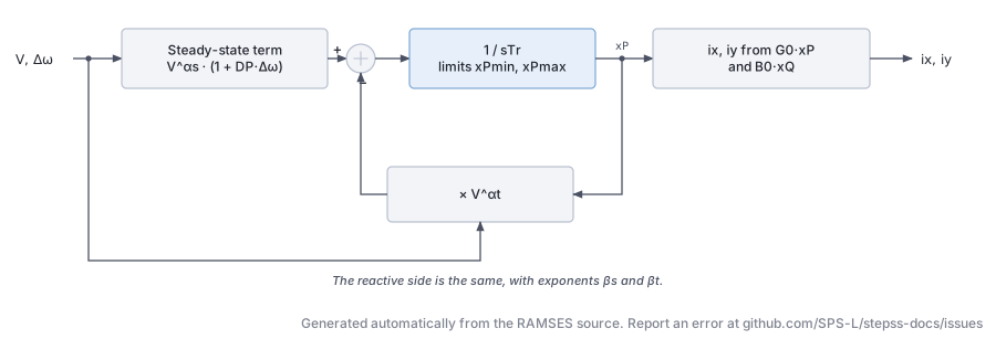
RESTLD (inj_restld): Restorative Load

Description

The restorative load model represents loads that self-restore toward a nominal characteristic after a voltage disturbance. The load’s active and reactive powers are governed by two internal recovery variables that evolve dynamically, allowing the simulation to capture the slow restoration of thermostatically controlled loads (heating, cooling) and similar self-restoring demand.

Scientific Description

The recovery variable $x_P$ for active power satisfies:

$\dot{x}_P = \frac{1}{T_r}\left[V^{\alpha_s}\left(1 + D_P\,\Delta\omega\right) - x_P\, V^{\alpha_t}\right]$

with analogous equation for $x_Q$. Here $\alpha_s$ and $\alpha_t$ are the steady-state and transient voltage exponents respectively. Limiters $[x_{P,\min},\, x_{P,\max}]$ are applied. The injected currents are expressed as:

$i_y = -B_0\left(1 + D_Q\,\Delta\omega\right) x_Q\, v_x + G_0\left(1 + D_P\,\Delta\omega\right) x_P\, v_y$

$i_x = \phantom{-}B_0\left(1 + D_Q\,\Delta\omega\right) x_Q\, v_y + G_0\left(1 + D_P\,\Delta\omega\right) x_P\, v_x$

where the ratio $V/V_0$ governs the voltage dependence through vrat.

Parameters

#	Name	Description	Unit
1	DP	Frequency sensitivity of active power	pu/pu
2	alphat	Transient active power voltage exponent
3	alphas	Steady-state active power voltage exponent
4	xP_min	Minimum limit for $x_P$
5	xP_max	Maximum limit for $x_P$
6	DQ	Frequency sensitivity of reactive power	pu/pu
7	betat	Transient reactive power voltage exponent
8	betas	Steady-state reactive power voltage exponent
9	xQ_min	Minimum limit for $x_Q$
10	xQ_max	Maximum limit for $x_Q$
11	Tr	Load recovery time constant	s

State Variables

Variable	Description
iy	$y$-component of injected current
ix	$x$-component of injected current
xp	Active power recovery variable
xq	Reactive power recovery variable

Observables: P, Q, xp, xq

Usage Example

INJEC  RESTLD  RESTLD1  BUS2  1.  1.  0.  0.  1.5  0.5  2.0  0.0  2.0  1.2  0.5  2.5  0.0  2.0  60.0  ;

---

PQ (inj_PQ): Constant PQ Load

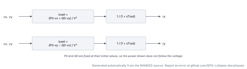
Description

The simplest injector model: maintains constant active and reactive power consumption regardless of bus voltage or frequency. The power is fixed at its initial operating-point value. A small first-order filter (time constant Tout) drives the injected currents smoothly to their target values, preventing algebraic loops.

Scientific Description

The current references are set to deliver the initial powers $P_0$ and $Q_0$ at the measured voltage $V$:

$I_{x,\mathrm{set}} = \frac{P_0 v_x + Q_0 v_y}{V^2}, \qquad I_{y,\mathrm{set}} = \frac{P_0 v_y - Q_0 v_x}{V^2}$

These references pass through a first-order filter with time constant $T_{\mathrm{out}}$ to produce the actual injected currents:

$T_{\mathrm{out}}\,\dot{i}_x + i_x = I_{x,\mathrm{set}}, \qquad T_{\mathrm{out}}\,\dot{i}_y + i_y = I_{y,\mathrm{set}}$

Parameters

#	Name	Description	Unit
1	Tout	Output filter time constant (recommended: 0.01 s)	s

Initial conditions $P_0$, $Q_0$, $V_0$ are computed automatically at initialization.

State Variables

Variable	Description
ix	Injected $x$-current
iy	Injected $y$-current
Ixset	Current reference $x$
Iyset	Current reference $y$
P	Observed active power
Q	Observed reactive power
V	Bus voltage magnitude

Observables: P, Q

Usage Example

INJEC  inj_PQ  LOAD_PQ  BUS3  1.  1.  0.  0.  0.01  ;

---

THEVEQ (inj_theveq): Thévenin Equivalent

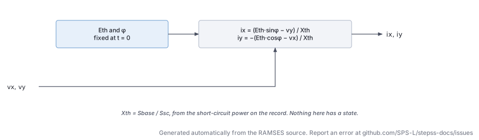
Description

Models an external network or generator cluster as a Thévenin equivalent: an ideal voltage source $\bar{E}_{\mathrm{th}}$ behind a pure reactance $X_{\mathrm{th}}$. The model computes the internal voltage magnitude and phase angle at initialization from the initial bus conditions and holds them constant during the simulation. It is useful for representing neighbouring system equivalents or simplified machine representations.

Scientific Description

The Thévenin reactance is obtained from the specified short-circuit power $S_{\mathrm{sc}}$ (MVA):

$X_{\mathrm{th}} = \frac{S_{\mathrm{base}}}{S_{\mathrm{sc}}}$

The internal voltage phasor is computed at $t=0$:

$E_{\mathrm{th},x} = v_x - X_{\mathrm{th}}\, i_y, \qquad E_{\mathrm{th},y} = v_y + X_{\mathrm{th}}\, i_x$

$E_{\mathrm{th}} = \sqrt{E_{\mathrm{th},x}^2 + E_{\mathrm{th},y}^2}, \qquad \phi = \arctan\!\left(\frac{E_{\mathrm{th},y}}{E_{\mathrm{th},x}}\right)$

During simulation the injected currents satisfy:

$i_y = -\frac{E_{\mathrm{th}}\cos\phi - v_x}{X_{\mathrm{th}}}, \qquad i_x = \frac{E_{\mathrm{th}}\sin\phi - v_y}{X_{\mathrm{th}}}$

Parameters

#	Name	Description	Unit
1	XTH	Short-circuit power of the equivalent (converted to $X_{\mathrm{th}}$ at initialization)	MVA

Internal parameters ETH (Thévenin voltage magnitude, pu) and phase (internal angle, rad) are computed automatically.

State Variables

Variable	Description
iy	Injected $y$-current
ix	Injected $x$-current

Observables: P, Q (in MW and Mvar at system base)

Usage Example

INJEC  THEVEQ  EQUIV1  SLACK_BUS  1.  1.  0.  0.  2000.0  ;

---

Induction Machine Models

INDMACH1 (inj_indmach1): Single-Cage Induction Machine

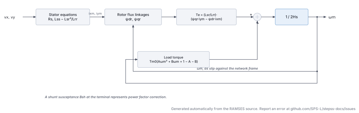
Description

A single-cage (single-rotor-circuit) induction machine model for motor loads. The machine is represented on its own MVA base (or inferred from load factor LF) with a shunt capacitor $B_{\mathrm{sh}}$ to represent power factor correction. The mechanical torque is a quadratic function of rotor speed. At initialization, the model solves nonlinear algebraic equations to find the operating-point slip and flux linkages.

Scientific Description

The machine uses the standard $d$-$q$ reference-frame formulation with $L_{ss} = L_{sr} + L_{ls}$ and $L_{rr} = L_{sr} + L_{lr}$. The rotor flux-linkage equations are:

$\frac{d\psi_{dr}}{dt} = \omega_0\left(-\frac{R_r}{L_{rr}}\psi_{dr} + \frac{L_{sr} R_r}{L_{rr}} i_{ym} - (\omega - \omega_m)\psi_{qr}\right)$

$\frac{d\psi_{qr}}{dt} = \omega_0\left(-\frac{R_r}{L_{rr}}\psi_{qr} + \frac{L_{sr} R_r}{L_{rr}} i_{xm} + (\omega - \omega_m)\psi_{dr}\right)$

where $\omega_0 = 2\pi f_{\mathrm{nom}}$ and $\omega_m$ is the rotor mechanical speed. The equations for the stator (with shunt susceptance $B_{\mathrm{sh}}$) are:

$R_s i_{ym} + \left(L_{ss} - \frac{L_{sr}^2}{L_{rr}}\right)\omega\, i_{xm} + \frac{L_{sr}}{L_{rr}}\omega\,\psi_{qr} = v_y$

$R_s i_{xm} - \left(L_{ss} - \frac{L_{sr}^2}{L_{rr}}\right)\omega\, i_{ym} - \frac{L_{sr}}{L_{rr}}\omega\,\psi_{dr} = v_x$

The rotor speed dynamics follow the swing equation:

$\frac{d\omega_m}{dt} = \frac{T_e - T_m}{2H}$

where the electromagnetic torque is:

$T_e = \frac{L_{sr}}{L_{rr}}\left(-\psi_{dr} i_{xm} + \psi_{qr} i_{ym}\right)$

and the mechanical torque is the quadratic load curve:

$T_m = T_{m0}\left(A\,\omega_m^2 + B\,\omega_m + 1 - A - B\right)$

Parameters

#	Name	Description	Unit
1	SNOM	Machine nominal apparent power (0 = infer from LF)	MVA
2	RS	Stator resistance	pu
3	Lls	Stator leakage inductance	pu
4	LSR	Magnetizing inductance	pu
5	RR	Rotor resistance	pu
6	Llr	Rotor leakage inductance	pu
7	H	Machine inertia constant	s
8	A	Quadratic torque-speed coefficient
9	B	Linear torque-speed coefficient
10	LF	Load factor (for SNOM inference)

State Variables

Variable	Description
iy	$y$-component of stator current
ix	$x$-component of stator current
psidr	$d$-axis rotor flux linkage
psiqr	$q$-axis rotor flux linkage
omegam	Rotor mechanical speed

Observables: P, Qmot+comp, Qmot, omega, Tm

Usage Example

INJEC  INDMACH1  MTR1  BUS_MV  1.  1.  0.  0.  10.0  0.01  0.10  2.50  0.015  0.10  1.5  0.8  0.1  0.0  ;

---

INDMACH2 (inj_indmach2): Double-Cage Induction Machine

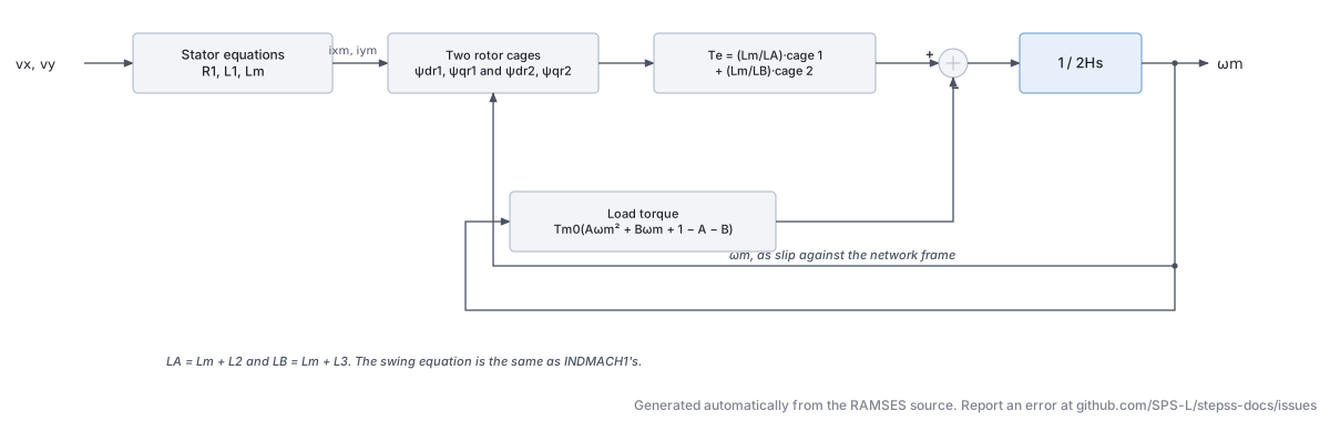
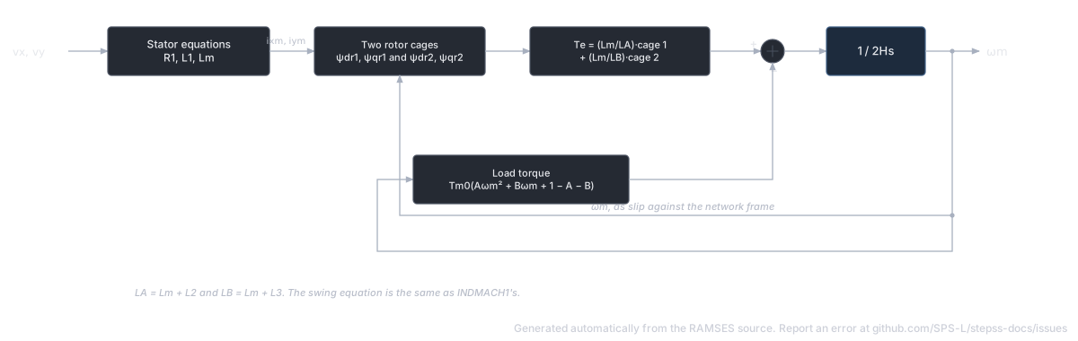
Description

A double-cage (double-rotor-circuit) induction machine model following the Eurostag formulation. Two parallel rotor cages allow more accurate representation of the machine’s impedance-vs-frequency characteristic, which is especially important for the starting transient. The model structure mirrors inj_indmach1 but includes a second set of rotor flux states.

Scientific Description

The machine has parameters: stator resistance $R_1$, stator leakage $L_1$, magnetizing inductance $L_m$, cage-1 resistance $R_2$ and leakage $L_2$, cage-2 resistance $R_3$ and leakage $L_3$. The state vector is $(\psi_{dr1},\psi_{qr1},\psi_{dr2},\psi_{qr2},\omega_m)$ with flux-linkage equations for each cage:

$\frac{d\psi_{dr1}}{dt} = \omega_0\left(-\frac{R_2}{L_{A}}\psi_{dr1} + \frac{L_m R_2}{L_{A}} i_{ym} - (\omega - \omega_m)\psi_{qr1}\right)$

$\frac{d\psi_{dr2}}{dt} = \omega_0\left(-\frac{R_3}{L_{B}}\psi_{dr2} + \frac{L_m R_3}{L_{B}} i_{ym} - (\omega - \omega_m)\psi_{qr2}\right)$

where $L_A = L_m + L_2$ and $L_B = L_m + L_3$. The total electromagnetic torque combines contributions from both cages:

$T_e = \frac{L_m}{L_A}\left(-\psi_{dr1} i_{xm} + \psi_{qr1} i_{ym}\right) + \frac{L_m}{L_B}\left(-\psi_{dr2} i_{xm} + \psi_{qr2} i_{ym}\right)$

The swing equation is identical to inj_indmach1.

Parameters

#	Name	Description	Unit
1	SNOM	Machine MVA rating (0 = infer from LF)	MVA
2	R1	Stator resistance	pu
3	L1	Stator leakage inductance	pu
4	Lm	Magnetizing inductance	pu
5	R2	First cage resistance	pu
6	L2	First cage leakage inductance	pu
7	R3	Second cage resistance	pu
8	L3	Second cage leakage inductance	pu
9	H	Inertia constant	s
10	A	Quadratic torque-speed coefficient
11	B	Linear torque-speed coefficient
12	LF	Load factor (for SNOM inference)

State Variables

Variable	Description
iy	$y$-component of stator current
ix	$x$-component of stator current
psidr1	$d$-axis flux of first rotor cage
psiqr1	$q$-axis flux of first rotor cage
psidr2	$d$-axis flux of second rotor cage
psiqr2	$q$-axis flux of second rotor cage
omegam	Rotor mechanical speed

Observables: P, Qmot+comp, Qmot, omega

Usage Example

INJEC  INDMACH2  MTR2  BUS_MV  1.  1.  0.  0.  10.0  0.01  0.08  2.00  0.02  0.06  0.04  0.10  1.5  0.8  0.1  0.0  ;

---

INDM1 (inj_INDM1): Alternative Induction Machine

The data-file model name is INDM1 (or inj_INDM1).

Note

Callable since 3.79. Earlier releases compiled this model under no name, so a data file referring to it was rejected. For built-in single-cage motors, use INDMACH1 instead.

Description

An alternative single-cage induction machine model that uses the INI_indmach1 helper function for initialization. It is equivalent in physics to inj_indmach1 but implements the equations using RAMSES .txt-style model syntax with explicit state initialization calls. This can simplify parameterization when the helper function’s output is directly used.

Scientific Description

The model equations match those of inj_indmach1, whose block diagram applies here unchanged. The key distinction is the use of the INI_indmach1 function at parameter-evaluation time to pre-compute $B_{\mathrm{sh}}$, $T_{m0}$, and the initial flux linkages and rotor speed, rather than solving the initialization system in Fortran. With $L_{ss} = L_{sr} + L_{ls}$ and $L_{rr} = L_{sr} + L_{lr}$, the rotor flux equations are:

$\frac{d\psi_{dr}}{dt} = 2\pi f_0 \left[ -\frac{R_R}{L_{rr}}\psi_{dr} + \frac{L_{SR} R_R}{L_{rr}} i_{ym} - (\omega - \omega_m)\psi_{qr} \right]$

$\frac{d\psi_{qr}}{dt} = 2\pi f_0 \left[ -\frac{R_R}{L_{rr}}\psi_{qr} + \frac{L_{SR} R_R}{L_{rr}} i_{xm} + (\omega - \omega_m)\psi_{dr} \right]$

The rotor speed integral uses:

$\frac{d\omega_m}{dt} = \frac{1}{2H}\left[\frac{L_{SR}}{L_{rr}}(-\psi_{dr} i_{xm} + \psi_{qr} i_{ym}) - T_{m0}(A\omega_m^2 + B\omega_m + 1 - A - B)\right]$

with a lower limit of $\omega_m \ge 0$.

Parameters

#	Name	Description	Unit
1	SNOM	Machine MVA rating	MVA
2	RS	Stator resistance	pu
3	Lls	Stator leakage inductance	pu
4	LSR	Magnetizing inductance	pu
5	RR	Rotor resistance	pu
6	Llr	Rotor leakage inductance	pu
7	H	Inertia constant	s
8	A	Quadratic torque-speed coefficient
9	B	Linear torque-speed coefficient
10	LF	Load factor

Computed internally: BSH (shunt susceptance), TM0 (initial mechanical torque), LSS, LRR.

State Variables

Variable	Description
Psidr	$d$-axis rotor flux linkage
Psiqr	$q$-axis rotor flux linkage
omegam	Rotor mechanical speed
iym, ixm	Stator current components (on machine base)
dPsidr, dPsiqr, domegam	Time-derivative auxiliary states

Observables: omegam

Usage Example

INJEC  INDM1  MTR3  BUS_MV  1.  1.  0.  0.  10.0  0.01  0.10  2.50  0.015  0.10  1.5  0.8  0.1  0.0  ;

---

Renewable Generation / Inverter-Based Resources

IBG (inj_IBG): Inverter-Based Generator (Generic IBR)

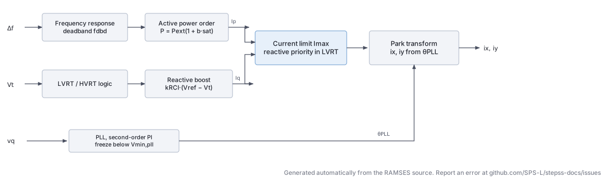
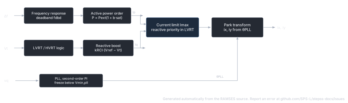
Description

A generic inverter-based generation model suitable for representing aggregated distributed generation or any grid-following IBR. The model includes a Phase-Locked Loop (PLL), inner current control with active ($I_p$) and reactive ($I_q$) current commands, LVRT/HVRT logic with voltage-dependent reactive current injection, frequency-responsive active power modulation, and reconnection logic after disconnection events.

Scientific Description

The PLL tracks the terminal voltage angle $\theta$ via a second-order PI controller with a freeze option below $V_{\mathrm{min,pll}}$:

$\frac{d\theta_{\mathrm{PLL}}}{dt} = \Delta\omega_{\mathrm{PLL}}, \qquad \frac{d\Delta\omega_{\mathrm{PLL}}}{dt} = k_{\mathrm{PLL}}\, v_q$

where $v_q$ is the $q$-axis terminal voltage in the PLL frame. The current commands $I_{p,\mathrm{cmd}}$ and $I_{q,\mathrm{cmd}}$ are derived from outer controls:

• Active power is modulated by frequency according to frequency deadband fdbd: $P = P_{\mathrm{ext}}\left(1 + b\,\mathrm{sat}(\Delta f - f_{\mathrm{start}}, f_{\mathrm{min}}, f_{\mathrm{max}})\right)$

• During voltage dips (LVRT), reactive current is boosted: $I_{q,\mathrm{boost}} = k_{\mathrm{RCI}}\,(V_{\mathrm{ref}} - V_t)$

• Current magnitude is limited to $I_{\mathrm{max}}$ with priority to reactive current during LVRT.

The injected currents in $x$-$y$ frame are:

$i_x = I_p \cos\theta_{\mathrm{PLL}} - I_q \sin\theta_{\mathrm{PLL}}$ $i_y = I_p \sin\theta_{\mathrm{PLL}} + I_q \cos\theta_{\mathrm{PLL}}$

Parameters

#	Name	Description	Unit
1	Imax	Maximum current magnitude	pu
2	IN	Nominal current	pu
3	Iprate	Active current ramp rate	pu/s
4	Tg	Generator time constant	s
5	Tm	Measurement filter time constant	s
6	tLVRT1	LVRT ride-through time threshold 1	s
7	tLVRT2	LVRT ride-through time threshold 2	s
8	tLVRTint	LVRT integration time	s
9	Vmax	Maximum voltage for operation	pu
10	tau	PLL response time	ms
11	Vminpll	Voltage below which PLL is frozen	pu
12	a	LVRT voltage-current curve slope
13	Vmin	Minimum LVRT voltage	pu
14	Vint	Intermediate LVRT voltage	pu
15	fmin	Minimum frequency for operation	pu
16	fmax	Maximum frequency for operation	pu
17	fstart	Frequency threshold for P modulation	pu
18	b	Frequency droop gain
19	fr	Reference frequency	pu
20	Tr	Reconnection delay after trip	s
21	Re	Grid equivalent resistance	pu
22	Xe	Grid equivalent reactance	pu
23	CM1	LVRT control mode flag
24	kRCI	Reactive current injection gain (LVRT)
25	kRCA	Reactive current absorption gain (HVRT)
26	m	Active-reactive current priority parameter
27	n	Active-reactive current priority parameter
28	dbmin	Frequency deadband lower limit	pu
29	dbmax	Frequency deadband upper limit	pu
30	HVRT	HVRT flag
31	LVRT	LVRT flag
32	CM2	Control mode 2 flag
33	Vtrip	Trip voltage threshold	pu

State Variables

Variable	Description
vxl, vyl	Filtered terminal voltage components
Vt	Terminal voltage magnitude
PLLPhaseAngle	PLL phase angle
Vm	Voltage magnitude measurement
Ip, Iq	Active and reactive current outputs
Ipcmd, Iqcmd	Current commands
Iqmax, Iqmin	Reactive current limits
Ipmax, Ipmin	Active current limits
DeltaW, DeltaWf	Frequency deviation and filtered value
Pgen, Qgen	Generated active and reactive power

Usage Example

INJEC  IBG  IBG1  BUS_GEN  1.  1.  0.  0.  1.2  1.0  0.5  0.02  0.01  0.5  1.0  0.05
                            1.1  20.0  0.1  2.0  0.1  0.5  0.95  1.05
                            0.0  2.0  1.0  1.0  0.0  0.05  1  2.0  1.5
                            2.0  2.0  -0.02  0.02  1  1  1  0.85  ;

---

WT3 (inj_WT3): Type 3 Wind Turbine (DFIG)

The data-file model name is WT3 (or inj_WT3).

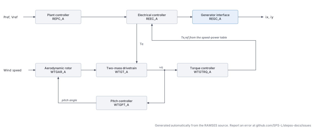
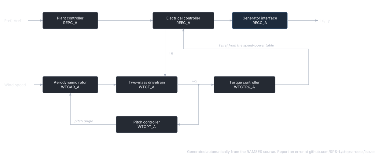
Description

A Type 3 wind turbine model implementing the WECC composite structure with four coupled sub-models:

• REPC_A: Plant-level controller (reactive power / voltage regulation, frequency response)
• REEC_A: Electrical controller (inner $d$-$q$ current control, LVRT/HVRT logic)
• WTGTRQ_A: Generator torque controller (rotor speed regulation via electrical torque command)
• WTGPT_A: Pitch controller (aerodynamic power limitation)
• WTGAR_A: Aerodynamic rotor model
• WTGT_A: Two-mass mechanical drivetrain (turbine inertia $H_t$, generator inertia $H_g$, shaft stiffness $K_{\mathrm{shaft}}$, damping $D_{\mathrm{shaft}}$)

The doubly-fed induction generator (DFIG) topology allows decoupled control of active and reactive power via rotor-side converter injection.

Scientific Description

The two-mass drivetrain model governs rotor dynamics:

$2H_t \frac{d\omega_t}{dt} = T_m - K_{\mathrm{shaft}}(\theta_t - \theta_g) - D_{\mathrm{shaft}}(\omega_t - \omega_g)$

$2H_g \frac{d\omega_g}{dt} = K_{\mathrm{shaft}}(\theta_t - \theta_g) + D_{\mathrm{shaft}}(\omega_t - \omega_g) - T_e$

The torque controller (WTGTRQ_A) uses a piecewise power-speed characteristic:

$T_{e,\mathrm{ref}} = \mathrm{interp}(\omega_g;\; [(\mathrm{spd}_1, p_1), (\mathrm{spd}_2, p_2), (\mathrm{spd}_3, p_3), (\mathrm{spd}_4, p_4)])$

The electrical controller (REEC_A) provides reactive current injection during voltage dips:

$I_{q,\mathrm{vdip}} = k_{qv}\left(V_{\mathrm{ref0}} - V_t\right)\quad \text{when } V_t < V_{\mathrm{dip}}$

with limiter $[I_{ql1}, I_{qh1}]$.

The plant controller (REPC_A) optionally provides frequency response:

$\Delta P_{\mathrm{ref}} = D_{\mathrm{dn}}\,\mathrm{sat}(\Delta f, f_{\mathrm{dbd1}}, 0) + D_{\mathrm{up}}\,\mathrm{sat}(\Delta f, 0, f_{\mathrm{dbd2}})$

Network interface. REGC_A injects a current rather than a voltage behind an impedance. The filtered active and reactive current commands $I_{pf}$, $I_{qf}$ are resolved into the network frame with the PLL angle and rescaled from the machine rating to the system base:

$i_x = \left(I_{pf}\cos\theta_{\mathrm{pll}} + I_{qf}\sin\theta_{\mathrm{pll}}\right)\frac{S_{\mathrm{nom}}}{S_{\mathrm{base}}}$

$i_y = \left(I_{pf}\sin\theta_{\mathrm{pll}} - I_{qf}\cos\theta_{\mathrm{pll}}\right)\frac{S_{\mathrm{nom}}}{S_{\mathrm{base}}}$

The PLL angle itself tracks the $q$-axis component of the filtered terminal voltage:

$v_q = -v_{x,\mathrm{filt}}\sin\theta_{\mathrm{pll}} + v_{y,\mathrm{filt}}\cos\theta_{\mathrm{pll}}$

WT4 and BESS use the same interface.

Parameters (selected key parameters)

#	Name	Sub-model	Description	Unit
1	SNOM		Nominal power	MW
2–32	REPC_A	Plant controller	Reactive/voltage/frequency control	various
33–46	WTGTRQ_A	Torque ctrl	Speed-torque lookup table, rate limits	various
47–56	WTGPT_A	Pitch ctrl	Pitch PI gains, angle limits, rate limits	various
57–58	WTGAR_A	Aero	Aerodynamic gain, initial pitch angle
59–62	WTGT_A	Drivetrain	$H_t$, $H_g$, $D_{\mathrm{shaft}}$, $K_{\mathrm{shaft}}$	s, pu
63–97	REEC_A	Elec ctrl	LVRT/HVRT, current limits, inner PI	various
98+	REGC_A	Generator	Generator electrical conversion	various

Full parameter list has 80+ entries; refer to a working example data file for the complete ordering.

Usage Example

INJEC  WT3  WT3_1  BUS_WIND  1.  1.  0.  0.
    100.0  0.0  0.02  0  0.0  0.05  0  0.0  0.3  -0.3  2.0  0.4  0.3  -0.3  0.0  0.15  0.9  0.05
    0.0  -0.06  0.06  -0.05  0.05  0.05  -0.05  2.0  1.0  1.0  -1.0  0.02  0  0  0.8
    1.5  1.5  0.01  0.5  ... ;

---

WT4 (inj_WT4): Type 4 Wind Turbine (Full Converter)

The data-file model name is WT4 (or inj_WT4).

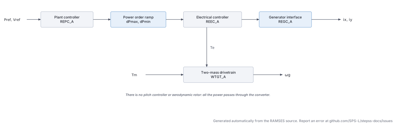
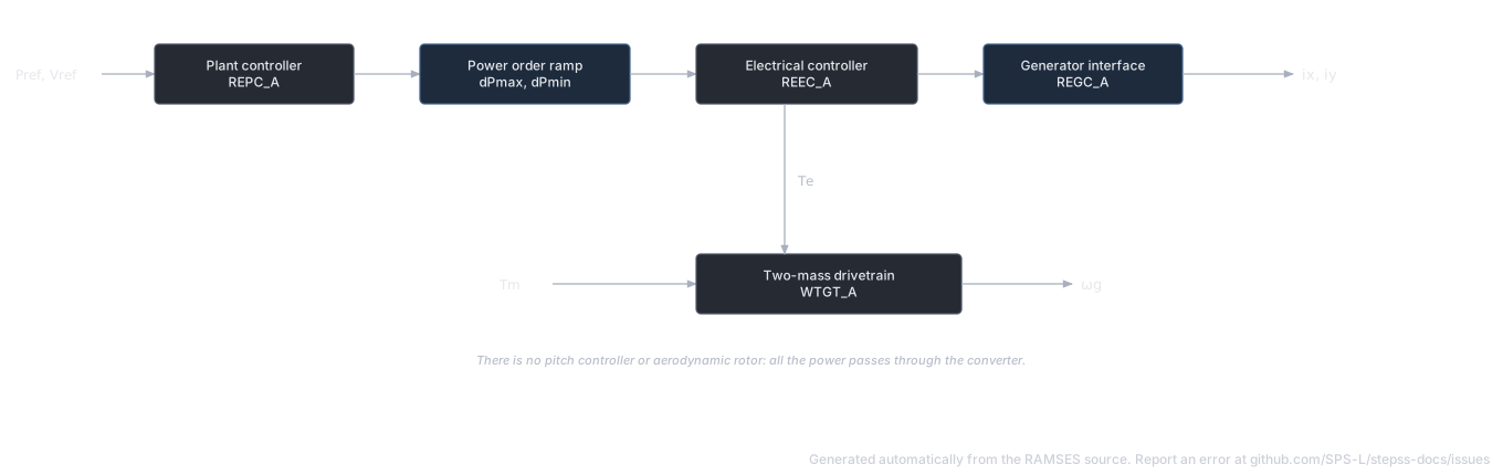
Description

A Type 4 wind turbine with full-rated converter. Unlike Type 3, the generator is fully decoupled from the grid through a back-to-back converter. The model implements the same WECC framework as WT3 but without the doubly-fed rotor circuit: the mechanical sub-model is a single-mass (or two-mass) drive train, and all electrical power passes through the converter. Sub-models include REPC_A (plant controller), REEC_A (electrical controller), WTGT_A (drivetrain), and REGC_A (generator/converter).

Scientific Description

The two-mass drivetrain is identical to WT3:

$2H_t \frac{d\omega_t}{dt} = T_m - K_{\mathrm{shaft}}\delta_{\mathrm{shaft}} - D_{\mathrm{shaft}}(\omega_t - \omega_g)$

$2H_g \frac{d\omega_g}{dt} = K_{\mathrm{shaft}}\delta_{\mathrm{shaft}} + D_{\mathrm{shaft}}(\omega_t - \omega_g) - T_e$

$\frac{d\delta_{\mathrm{shaft}}}{dt} = \omega_0(\omega_t - \omega_g)$

There is no pitch controller or aerodynamic rotor in the basic Type 4 configuration; the active power reference is supplied directly (or from REPC_A), and rate limits dPmax/dPmin apply to the power order ramp.

The REEC_A electrical controller supplies current commands with the same LVRT/HVRT logic as WT3, with current limits through the converter lookup table (piecewise linear in voltage: $(V_{p1}, I_{p1}),\ldots,(V_{p4}, I_{p4})$ for active current and $(V_{q1}, I_{q1}),\ldots,(V_{q4}, I_{q4})$ for reactive).

Parameters (selected key parameters)

#	Name	Sub-model	Description	Unit
1	SNOM		Nominal power	MW
2–32	REPC_A	Plant ctrl	Same as WT3	various
33–37	WTGT_A	Drivetrain	$H_t$, $H_g$, $\omega_0$, $D_{\mathrm{shaft}}$, $K_{\mathrm{shaft}}$	s, pu
38–80	REEC_A	Elec ctrl	LVRT, current limits, PI gains	various
81+	REGC_A	Generator	Converter electrical model	various

Usage Example

INJEC  WT4  WT4_1  BUS_WIND  1.  1.  0.  0.
    100.0  0.0  0.02  0  0.0  0.05  0  0.0  0.3  -0.3  2.0  0.4  0.3  -0.3  0.0  0.15  0.9  0.05
    0.0  -0.06  0.06  -0.05  0.05  0.05  -0.05  2.0  1.0  1.0  -1.0  0.02  0  0  5.0  1.5  1.0  1.5  20.0  ... ;

---

PV (inj_PV): Photovoltaic Generator

The data-file model name is PV (or inj_PV).

Note

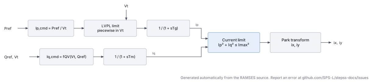
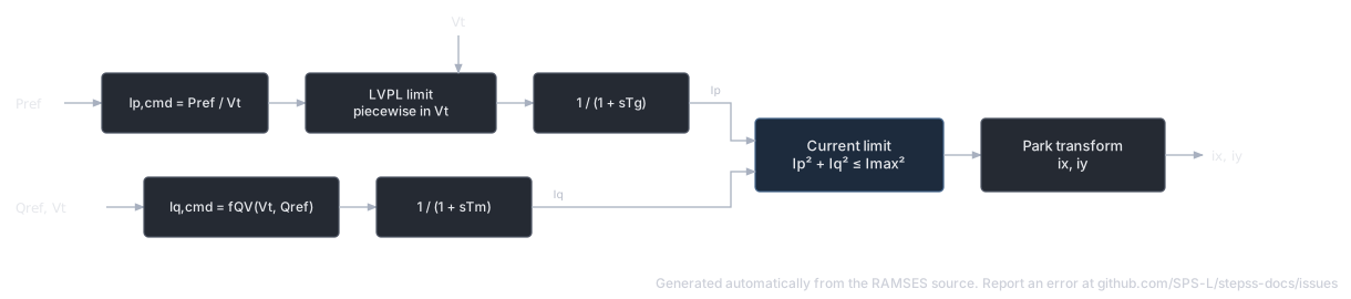
Callable since 3.79. Earlier releases compiled this model under no name, so a data file referring to it was rejected.

Description

A photovoltaic generator model with similar WECC-derived structure to the wind turbine models. The model includes a plant controller (voltage/reactive power regulation), an electrical controller (current limits, LVRT), and generator/converter representation. Unlike wind turbines, there is no mechanical drive train; the active power set-point follows an irradiance input or a fixed reference. LVRT/HVRT logic and current limiting are identical to the Type 4 wind model.

Scientific Description

The PV generator delivers active and reactive power through current commands:

$I_p = \frac{P_{\mathrm{ref}}}{V_t}, \qquad I_q = f_{\mathrm{QV}}(V_t, Q_{\mathrm{ref}})$

subject to the constraint $\sqrt{I_p^2 + I_q^2} \leq I_{\mathrm{max}}$. The inner current loop is a first-order filter:

$T_g \frac{dI_p}{dt} = I_{p,\mathrm{cmd}} - I_p, \qquad T_m \frac{dI_q}{dt} = I_{q,\mathrm{cmd}} - I_q$

Low-voltage power-logic (LVPL) limits active current during deep voltage sags via a piecewise-linear function of $V_t$ with breakpoints lvpnt0, lvpnt1, Lvpl1. HVRT and LVRT timers control disconnection and reconnection.

Parameters (selected)

#	Name	Description	Unit
1	Imax	Maximum converter current	pu
2	IN	Nominal current	pu
3	ratemax	Reconnection ramp rate	pu/s
4	Tg	Active current filter time constant	s
5	Tm	Reactive current filter time constant	s
6–9	LVRT timers	tLVRT1, tLVRT2, tLVRTint, Vmax	s, pu
10	kpll	PLL gain
11	Vminpll	PLL freeze voltage	pu
12–14	LVRT curve	a, Vmin, Vint
21–22	Re, Xe	Grid equivalent impedance	pu
23–29	Current control	CM1, kRCI, kRCA, m, n, dbmin, dbmax
34	BM	Battery module flag

Usage Example

INJEC  PV  PV1  BUS_PV  1.  1.  0.  0.  1.2  1.0  0.5  0.02  0.01  0.5  1.0  0.05  1.1
                          20.0  0.1  2.0  0.1  0.5  0.95  1.05  0.0  2.0  1.0
                          1.0  0.0  0.05  1  2.0  1.5  2.0  2.0  -0.02  0.02  1  1  1  0.85  0  ;

---

GFOR (inj_GFOR): Grid-Forming Converter (VSM)

The data-file model name is GFOR (or inj_GFOR).

Description

A grid-forming voltage source converter implementing Virtual Synchronous Machine (VSM) dynamics, modelled under the phasor approximation. The converter is an MMC-type VSC connected to the grid through its transformer (no LC filter); the DC side is not modelled (the DC voltage is assumed constant) so the focus is on the AC grid dynamics.

The modulated voltage magnitude is held at its setpoint $V_m^0$ in normal operation, while the phase angle $\delta_m$ is driven by a synthetic swing equation with inertia emulation ($H$) and oscillation damping ($D$) against a PLL estimate of the grid frequency. Participation in primary frequency control is optional, through the droop $R_{\mathrm{droop}}$. Overcurrents are limited by proportionally scaling the $d$-$q$ current vector back to the $I_{\mathrm{max}}$ circle with a small time constant.

Scientific Description

Reference frame. The $d$ axis is attached to the internal phase angle $\delta_m$ of the modulated voltage. Voltages and currents at the point of common coupling are transformed as:

$v_d = v_x\cos\delta_m + v_y\sin\delta_m, \qquad v_q = -v_x\sin\delta_m + v_y\cos\delta_m$

with the analogous transformation for the converter-side currents $i_{xt} = k\, i_x$, $i_{yt} = k\, i_y$, where $k = r\, S_{\mathrm{base}}/S_{\mathrm{nom}}$ converts to per-unit on the converter base.

Transformer. The voltage-current relationship across the connection transformer (resistance $R$, inductance $L$, ideal ratio $r$) in the $d$-$q$ frame is:

$v_{md} = \frac{v_d}{r} + R\, i_d - \omega_m L\, i_q, \qquad v_{mq} = \frac{v_q}{r} + R\, i_q + \omega_m L\, i_d$

PLL. The PLL only serves to estimate the grid angular frequency $\tilde{\omega}_g$ for the damping term. It is the same model as in the grid-following converter (see the PLL diagram there), with PI gains derived from the time constant $T_{\mathrm{pll}}$:

$K_{p\omega} = \frac{10}{\omega_N T_{\mathrm{pll}}}, \qquad K_{i\omega} = \frac{25}{\omega_N T_{\mathrm{pll}}^2}, \qquad \omega_N = 2\pi f_N$

The PLL is frozen (hysteresis) when the PCC voltage falls below 0.4 pu and reactivated when it recovers above 0.5 pu (fixed thresholds in this model).

Active power and phase angle control (VSM).

$2H\frac{d\omega_m}{dt} = P^* - P_{\mathrm{virt}} - D\left(\omega_m - \tilde{\omega}_g\right) + \frac{1 - \omega_m}{R_{\mathrm{droop}}}$

$\frac{d\delta_m}{dt} = \omega_N\left(\omega_m - \omega_{\mathrm{ref}}\right)$

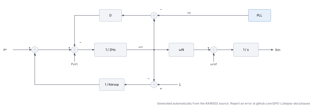
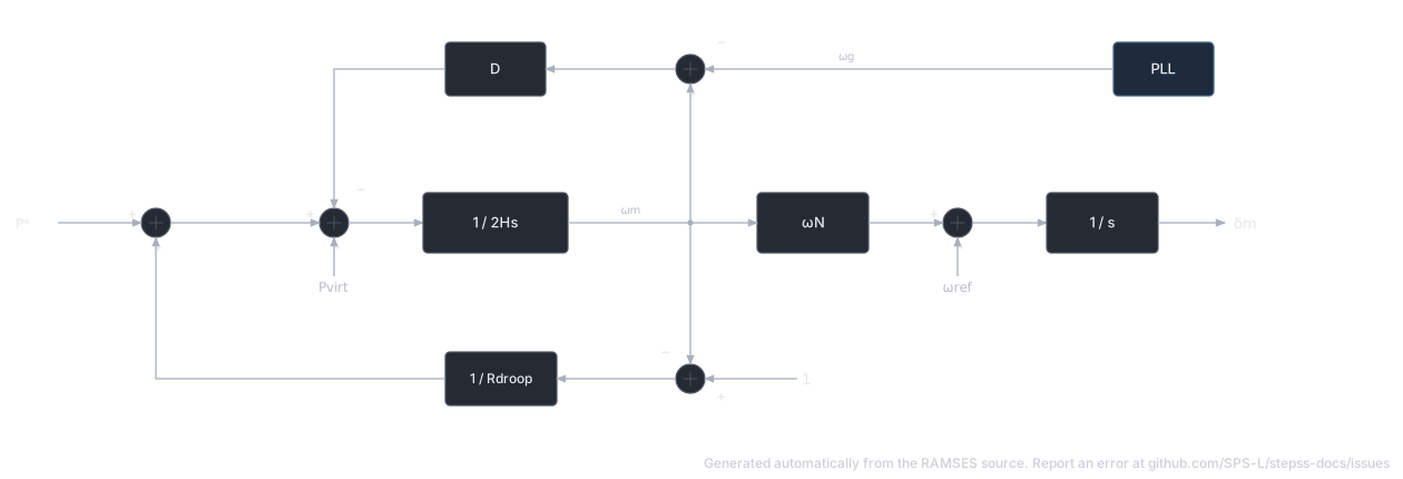
where $P^*$ is the active power setpoint and $P_{\mathrm{virt}}$ is the virtual power computed from the unsaturated currents:

$P_{\mathrm{virt}} = \frac{v_d}{r}\, i_d^* + \frac{v_q}{r}\, i_q^*$

$P_{\mathrm{virt}}$ equals the actual active power $P$ when the current is not limited, and yields improved large-disturbance stability while the current is limited (the angle dynamics do not wind up).

Current limitation. The currents $(i_d^*, i_q^*)$ that would result from normal voltage control (i.e. $v_{md} = V_m^0$, $v_{mq} = 0$) are first determined from:

$V_m^0 = \frac{v_d}{r} + R\, i_d^* - \omega_m L\, i_q^*, \qquad 0 = \frac{v_q}{r} + R\, i_q^* + \omega_m L\, i_d^*$

The current overload ratio $\rho = \sqrt{(i_d^*)^2 + (i_q^*)^2}\,/\,I_{\mathrm{max}}$ is passed through a first-order lag with time constant $T_e$ (typically 1 ms) and a non-windup lower limit of 1, giving $\rho_s$. Both current components are then decreased in the same proportion:

$i_{ds}^* = \frac{i_d^*}{\rho_s}, \qquad i_{qs}^* = \frac{i_q^*}{\rho_s}$

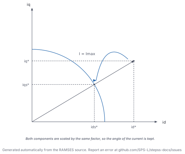
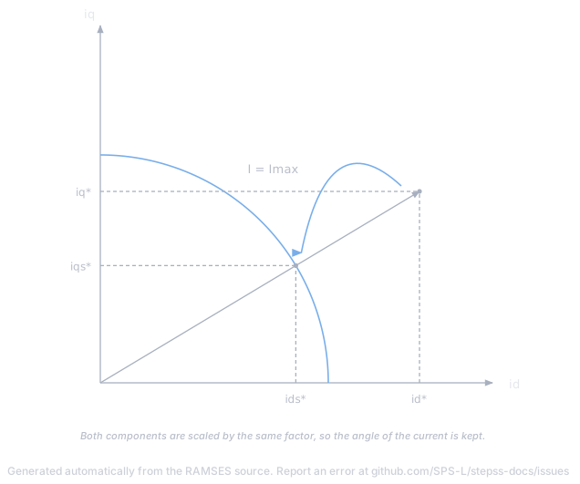
and the modulated voltage is set to the value that yields the saturated currents:

$v_{md} = \frac{v_d}{r} + R\, i_{ds}^* - \omega_m L\, i_{qs}^*, \qquad v_{mq} = \frac{v_q}{r} + R\, i_{qs}^* + \omega_m L\, i_{ds}^*$

When $I < I_{\mathrm{max}}$: $\rho_s = 1$, the currents are unsaturated, and $v_{md} = V_m^0$, $v_{mq} = 0$.

Parameters

Default values correspond to a 1100 MVA converter. Per-unit values refer to the nominal apparent power of the converter.

#	Name	Description	Unit	Default
1	R	Resistance of connection transformer	pu	0.005
2	L	Inductance of connection transformer	pu	0.15
3	r	Ratio of ideal transformer		1.02
4	Snom	Nominal apparent power	MVA	1100
5	H	Inertia constant	s	5.0
6	D	Damping constant of virtual synchronous machine		300
7	Tpll	Time constant of PLL	s	0.1
8	Rdroop	Droop of primary frequency control	pu	999
9	Imax	Maximum current (typically 1–1.2)	pu	1.0
10	Te	Time constant of current saturation	s	0.001

A very large Rdroop (e.g. 999) effectively disables participation in primary frequency control.

Five additional parameters are computed at initialization from the power-flow solution: k (current conversion factor), vmx0, vmy0 (components of the initial modulated voltage), Vmo (its magnitude $V_m^0$, i.e. the voltage setpoint) and Po (the active power setpoint $P^*$, pu on Snom base). Vmo and Po can be modified during the simulation with CHGPRM disturbances to change the voltage and active power setpoints.

State Variables

The model has 33 states (2 output currents + 31 internal). Key internal states:

Variable	Description	Unit
wref	Angular speed of reference axes	pu
ixt, iyt	Converter-side currents (on Snom base)	pu
Vm, deltam	Modulated voltage magnitude and phase angle	pu, rad
V	Voltage magnitude at PCC	pu
mult_pll	PLL freezing factor (hysteresis output)
w_pll, theta_pll	PLL frequency and angle estimates	pu, rad
P, Pvirt	Active power and virtual power (on Snom base)	pu
omegam	Angular frequency of modulated voltage	pu
vd, vq, id, iq	PCC voltage and current in $d$-$q$ frame	pu
id*, iq*	Unsaturated currents	pu
id*s, iq*s	Saturated currents	pu
rho, rhos	Current overload ratio and its saturated value
Q	Reactive power (on Snom base)	pu

Observables: P, Pvirt, Q, Vm, vmd, vmq, deltam, omegam, w_pll, I, id, id*, id*s, iq, iq*, iq*s, rho, rhos.

Usage Example

A 1100 MVA grid-forming converter:

#                 name   bus  FP   FQ   P   Q    R      L     r     Snom   H     D    Tpll  Rdroop Imax   Te
INJEC    GFOR     HVDC    A   1.   1.   0.  0.  0.005  0.15  1.02  1100.  5.0   300.  0.100  999.   1.0  0.001 ;

Note

At operating points where the initial current is below $I_{\mathrm{max}}$, RAMSES reports a small initial mismatch on the $\rho_s$ lag equation (“INJECTORS NOT IN STEADY STATE”). This is benign: $\rho_s$ starts exactly at its lower limit of 1 and is clamped there by the discrete update within the first time step.

---

GFOL (inj_GFOL): Grid-Following Converter

The data-file model name is GFOL (or inj_GFOL).

Description

A grid-following voltage source converter modelled under the phasor approximation. As for the grid-forming model, the converter is an MMC-type VSC connected through its transformer (no LC filter) and the DC side is not modelled. The model is rather detailed: it includes measurement low-pass filters, a PLL with blocking/unblocking hysteresis, outer active power and voltage/reactive power control loops, inner $d$-$q$ current control loops, a rate-limited $d$-axis current limit with priority to the reactive current, and a piecewise-linear dynamic voltage support characteristic.

Scientific Description

Reference frame. The VSC control frame $(d, q)$ tracks the PCC voltage phasor through the PLL angle $\tilde{\delta}_g$ (state theta_pll):

$v_d = v_x\cos\tilde{\delta}_g + v_y\sin\tilde{\delta}_g, \qquad v_q = -v_x\sin\tilde{\delta}_g + v_y\cos\tilde{\delta}_g$

with the analogous transformation for the converter-side currents ($i_{xt} = k\, i_x$, $k = r\, S_{\mathrm{base}}/S_{\mathrm{nom}}$). In steady state $v_q = 0$ and $v_d = V$.

Phase Locked Loop.

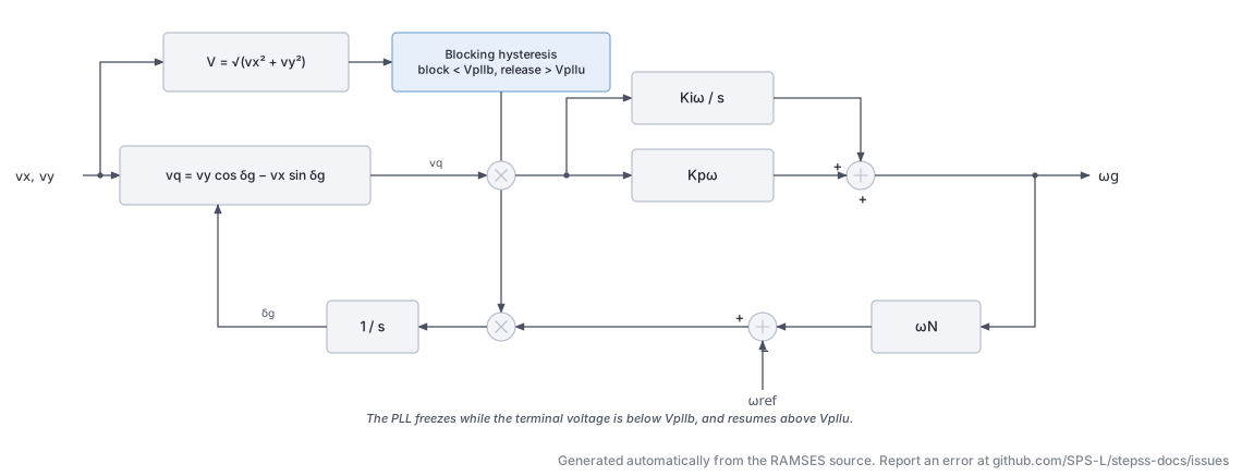
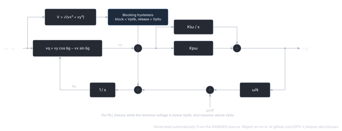
The $q$-axis voltage error drives a PI controller whose output is the grid frequency estimate $\tilde{\omega}_g$ (state w_pll); integrating $\omega_N(\tilde{\omega}_g - \omega_{\mathrm{ref}})$ gives the PLL angle. The PI gains follow from the PLL response time $\tau$:

$K_{p\omega} = \frac{10}{\omega_N \tau}, \qquad K_{i\omega} = \frac{25}{\omega_N \tau^2}, \qquad \omega_N = 2\pi f_N$

The PLL is blocked once the PCC voltage $V$ falls below Vpllb and reactivated once $V$ recovers above Vpllu (hysteresis).

Inner current control.

$v_{md} = \frac{v_d}{r} - \tilde{\omega}_g L\, i_q + \left(K_p + \frac{K_i}{s}\right)\left(i_d^{\mathrm{ref}} - i_d\right)$

$v_{mq} = \tilde{\omega}_g L\, i_d + \left(K_p + \frac{K_i}{s}\right)\left(i_q^{\mathrm{ref}} - i_q\right)$

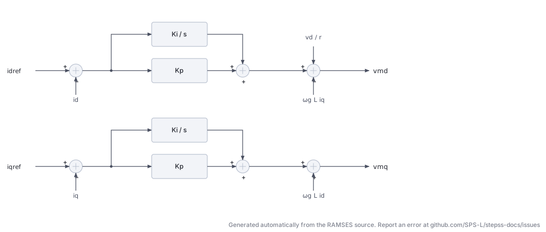
combined with the transformer voltage-current relationship in the $d$-$q$ frame:

$v_{md} = \frac{v_d}{r} + R\, i_d - \tilde{\omega}_g L\, i_q, \qquad v_{mq} = \frac{v_q}{r} + R\, i_q + \tilde{\omega}_g L\, i_d$

Active power control.

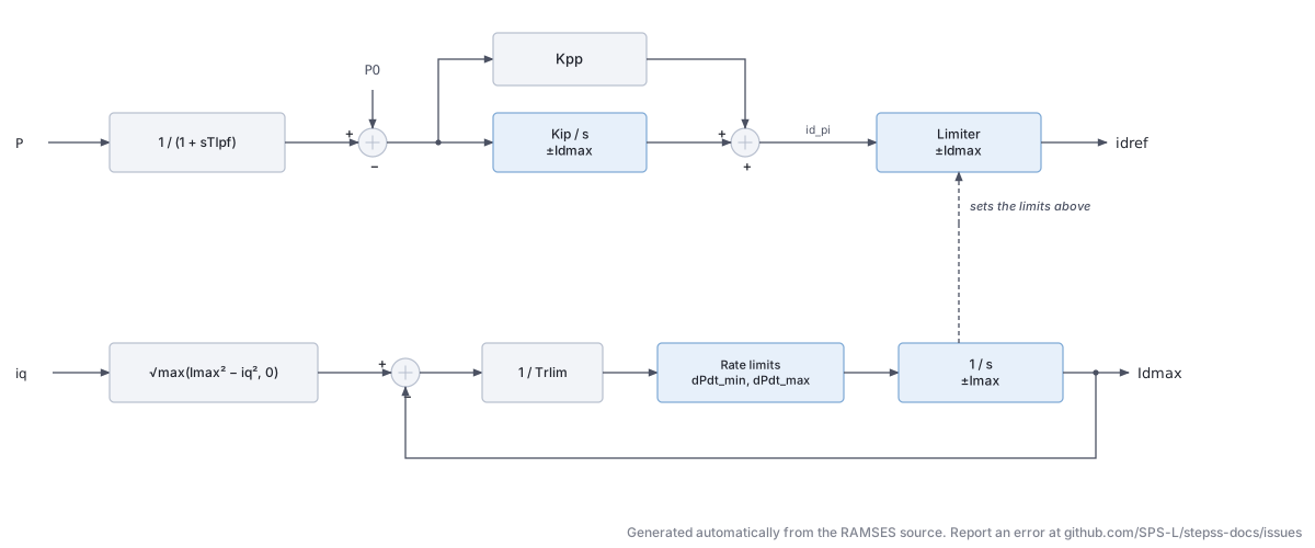
The measured active power is filtered with time constant $T_{\mathrm{lpf}}$ and compared with the setpoint $P^0$; a PI controller ($K_{pp}$, $K_{ip}$) with non-windup limits $\pm I_d^{\max}$ produces $i_d^{\mathrm{ref}}$. The limit gives priority to the reactive current:

$I_d^{\max,\mathrm{stat}} = \sqrt{\max\left(I_{\mathrm{max}}^2 - i_q^2,\; 0\right)}$

and $I_d^{\max}$ tracks this static value through a first-order lag ($T_{\mathrm{rlim}}$, typically 0.002 s) with rate limits dPdt_min/dPdt_max, limiting in particular the rate of recovery of the active current after it has been decreased by an increase of $i_q$.

Voltage / reactive power control.

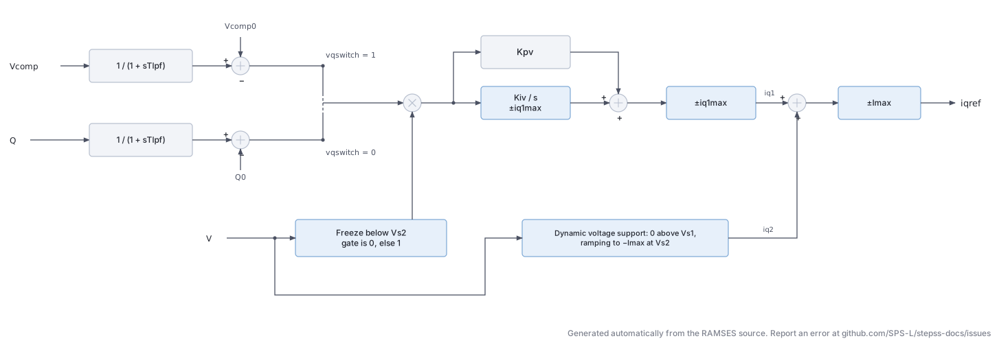
Depending on vqswitch, either the compensated voltage or the reactive power is controlled:

$V_c = \left|\frac{\bar{v}}{r} + (R_c + jX_c)\,\bar{i}\right| \quad (\texttt{vqswitch}=1), \qquad Q = \frac{v_q}{r} i_d - \frac{v_d}{r} i_q \quad (\texttt{vqswitch}=0)$

The controlled quantity is filtered ($T_{\mathrm{lpf}}$) and its deviation from setpoint drives a PI controller ($K_{pv}$, $K_{iv}$) with non-windup limits $\pm i_{q1}^{\max}$, giving the component $i_{q1}$. The error is zeroed (controller frozen) while $V < V_{s2}$. A second component $i_{q2}$ implements dynamic voltage support as a piecewise-linear function of $V$: zero above $V_{s1}$, decreasing linearly to $-I_{\mathrm{max}}$ at $V_{s2}$, constant below. The total $i_{q1} + i_{q2}$, limited to $\pm I_{\mathrm{max}}$, is the reactive current reference $i_q^{\mathrm{ref}}$.

With $R_c = R$, $X_c = \omega L$ and $r = 1$, controlling $V_c$ amounts to controlling the magnitude of the modulated voltage.

Parameters

Default values correspond to a 1200 MVA converter. Per-unit values refer to the nominal apparent power of the converter.

#	Name	Description	Unit	Default
1	R	Phase reactor resistance	pu	0.005
2	L	Phase reactor inductance	pu	0.15
3	r	Ratio of ideal transformer		1.02
4	Snom	Nominal apparent power	MVA	1200
5	Rc	Resistance used in compensated voltage	pu	0.005
6	Xc	Reactance used in compensated voltage	pu	0.15
7	Kp	Current control: proportional gain		0.573
8	Ki	Current control: integral gain		6.0
9	Tlpf	Measurement time constant (low-pass filter)	s	0.0033
10	Kpp	Active power control: proportional gain		0.0333
11	Kip	Active power control: integral gain		10.0
12	Trlim	Time constant of the $I_d^{\max}$ rate limiter	s	0.002
13	dPdt_min	Min rate of change of the $d$-current limit	pu/s	-999
14	dPdt_max	Max rate of change of the $d$-current limit	pu/s	10.0
15	Kpv	Reactive power control: proportional gain		0.1667
16	Kiv	Reactive power control: integral gain		50.0
17	tau	Response time of PLL	s	0.10
18	Vpllb	Voltage below which the PLL is blocked	pu	0.4
19	Vpllu	Voltage above which the PLL is unblocked	pu	0.5
20	Imax	Maximum current (typically 1–1.2)	pu	1.0
21	Vs1	Voltage below which dynamic reactive support starts	pu	-1000
22	Vs2	Voltage at which reactive support is maximum ($V_{s2} < V_{s1}$)	pu	-2000
23	iqmax	Limit (±) on quadrature current component $i_{q1}$	pu	1.001
24	vqswitch	1 = voltage control, 0 = reactive power control	flag	1

Setting Vs1 and Vs2 to large negative values (as in the defaults above) disables the dynamic voltage support; a more elaborate control is recommended for that function. Typical values of Kiv are 50 pu/s for voltage control and 10 pu/s for reactive power control.

Six additional parameters are computed at initialization from the power-flow solution: k (current conversion factor), P0, Q0 (active/reactive power setpoints, pu on Snom base), Vc0 (compensated voltage setpoint), Imin and iq1max ($= \min(\texttt{iqmax}, I_{\mathrm{max}})$). P0, Q0 and Vc0 can be modified during the simulation with CHGPRM disturbances.

State Variables

The model has 52 states (2 output currents + 50 internal). Key internal states:

Variable	Description	Unit
wref	Angular speed of reference axes	pu
ixt, iyt	Converter-side currents (on Snom base)	pu
mult_pll	PLL freezing factor (hysteresis output)
w_pll, theta_pll	PLL frequency and angle estimates	pu, rad
V, vd, vq	PCC voltage magnitude and $d$-$q$ components	pu
id, iq	Converter currents in $d$-$q$ frame	pu
vmd, vmq	Modulated voltage components	pu
Md, Mq	Current-control PI outputs	pu
Idmax_stat, Idmax, Idmin	Static / rate-limited / minimum $d$-current limits	pu
P, Pfil	Active power and its filtered value	pu
id_pi, idref	Active-power PI output and $d$-current reference	pu
Vc, Vcfil	Compensated voltage and its filtered value	pu
Q, Qfil	Reactive power and its filtered value	pu
mult_V	Voltage/reactive controller freezing factor
iq_1, iq_2, iqref	Reactive current components and reference	pu

Observables: P_MW, Q_Mvar, Vc, Vm, vmd, vmq, I, w_pll, theta_pll_deg, mult_pll, Idmax, Md, idref, id, id_pi, iq_1, iq_2, iqref, iq.

Usage Example

A 1200 MVA grid-following converter (record spanning multiple lines):

#              name    bus  FP   FQ   P   Q    R      L      r     Snom    Rc     Xc      Kp     Ki   Tlpf     Kpp    Kip   Trlim  dPdt_min dPdt_max  Kpv     Kiv
INJEC  GFOL    HVDC1    A   1.   1.   0.  0.  0.005  0.15   1.02   1200.  0.005   0.15   0.5730   6.  0.0033  0.0333   10.   0.002    -999.    10.    0.1667  50.
# tau   Vpllb  Vpllu   Imax    Vs1    Vs2    iq1max   vqswitch
  0.10    0.4    0.5   1.000   -1000  -2000  1.001        1     ;

---

Energy Storage

BESS (inj_BESS): Battery Energy Storage System

The data-file model name is BESS (or inj_BESS).

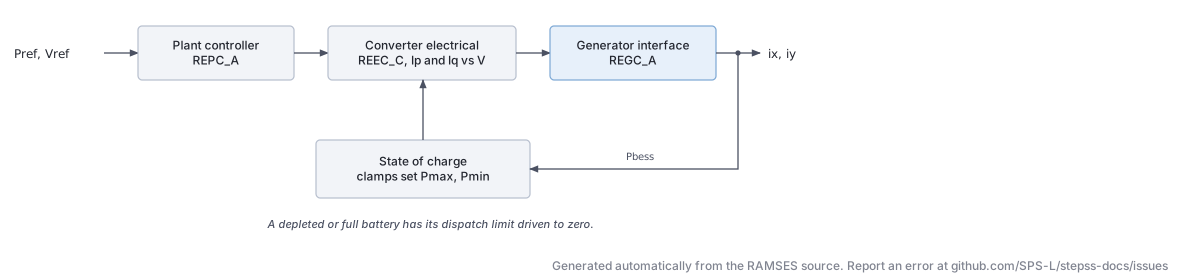
Description

A comprehensive BESS model implementing the full WECC framework (REPC_A + REEC_C + REGC_A) plus battery state of charge (SOC) tracking. The model supports both grid-following operation (bidirectional active power dispatch) and reactive power / voltage regulation. It is built on the same REPC_A plant controller as the wind turbine models, and uses the REEC_C converter electrical controller which handles a piecewise-linear $I_q$-vs-$V$ and $I_p$-vs-$V$ characteristic for fault ride-through.

The battery SOC evolves through integration of injected power:

$\frac{d\mathrm{SOC}}{dt} = -\frac{P_{\mathrm{bess}}}{C_{\mathrm{bat}} \cdot S_{\mathrm{nom}}}$

with hard clamps at SOCmin and SOCmax that modify the active power limits Pmax/Pmin dynamically:

$P_{\max} = \begin{cases} 0 & \mathrm{SOC} \ge \mathrm{SOC}_{\max}\\ P_{\max,\mathrm{rated}} & \text{otherwise}\end{cases}$

$P_{\min} = \begin{cases} 0 & \mathrm{SOC} \le \mathrm{SOC}_{\min}\\ P_{\min,\mathrm{rated}} & \text{otherwise}\end{cases}$

Parameters (key parameters)

#	Name	Sub-model	Description	Unit
1	SNOM		Nominal power	MW
2–32		REPC_A	Plant controller (same as WT3/WT4)	various
33–76		REEC_C	Electrical controller with piecewise $I_q(V)$, $I_p(V)$	various
68	CapBat	BESS	Battery energy capacity	MWh
69	SOCini	BESS	Initial state of charge	pu
70	SOCmax	BESS	Maximum SOC limit	pu
71	SOCmin	BESS	Minimum SOC limit	pu
72–73	dPmax, dPmin	BESS	Active power ramp rate limits	pu/s
74–75	pmax, pmin	REEC_C	Active current limits (pu on SNOM)	pu
76	Tpord	REEC_C	Active power order time constant	s

Full parameter listing has approximately 125 parameters; refer to a working example data file for the complete ordering.

State Variables

The BESS model uses over 40 internal states reflecting the three sub-models. Key states include:

Variable	Description
SOC	State of charge
Pref	Active power reference
Qext	Reactive power reference from REPC_A
Ip, Iq	Active/reactive current outputs
PLLPhaseAngle	PLL phase angle
Pgen, Qgen	Generated powers

Usage Example

INJEC  BESS  BESS1  BUS_ST  1.  1.  0.  0.
    100.0  0.0  0.02  0  0.0  0.05  0  0.0  0.3  -0.3  2.0  0.4
    0.3  -0.3  0.0  0.15  0.9  0.05  0.0  -0.06  0.06  -0.05  0.05
    0.05  -0.05  2.0  1.0  1.0  -1.0  0.02  0  0
    0.1  0.1  0.02  1.0  0.0  -0.2  0.2  0.2  -0.2  0.6  0.4  0.6  -0.6  1.1  0.9
    1.0  0.5  0.01  0.01  0.05  0.9  0.2  0.9  0.1  0.9  -0.1  0.5  -0.5  0.5  -0.5  1.0  -1.0  0.5  -0.5
    50.0  0.7  0.9  0.1  5.0  -5.0  1.0  -1.0  0.05  1.1  0.0  2  0.01  ;

---

Reactive Compensation

SVC_GENERIC1 (inj_svc_generic1): Generic Static Var Compensator

The data-file model name is SVC_GENERIC1. It takes no prefix.

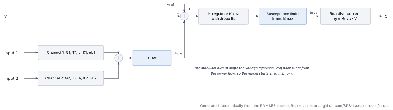
Description

A dynamic SVC injecting a purely reactive current at its bus. A PI voltage regulator with droop drives a susceptance $B_{svc}$ between Bmin and Bmax, and two lead-lag stabiliser channels can add a supplementary signal to the voltage reference. This is the dynamic counterpart of the static SVC record used by the power flow: the static record fixes the operating point, this model governs how the device behaves during the simulation.

The voltage reference is initialised from the power flow solution, so that the model starts in equilibrium:

$V_{ref} = V_0 + B_p \cdot B_{svc,0}$

where $B_p$ is the droop and $B_{svc,0}$ the initial susceptance implied by the reactive current at the bus.

Parameters

The record carries 17 data parameters, in order:

#	Name	Description
1	G1	Gain of the first stabiliser channel
2	T1	Time constant of the first stabiliser channel (s)
3	a	Lead-lag coefficient of the first channel
4	K1	Output gain of the first channel
5	L1	Output limit of the first channel (pu)
6	G2	Gain of the second stabiliser channel
7	T2	Time constant of the second stabiliser channel (s)
8	b	Lead-lag coefficient of the second channel
9	K2	Output gain of the second channel
10	L2	Output limit of the second channel (pu)
11	Ltot	Limit on the summed stabiliser output (pu)
12	Kp	Proportional gain of the voltage regulator
13	Ki	Integral gain of the voltage regulator
14	Bp	Droop, in pu on the SVC base
15	Bmax	Maximum susceptance (Mvar at 1 pu voltage)
16	Bmin	Minimum susceptance (Mvar at 1 pu voltage)
17	Bnom	Susceptance base used for the per-unit conversion (Mvar)

One additional parameter is computed at initialisation:

#	Name	Description
18	Vref	Voltage reference, set from the power flow solution

Observables

Q, dvpss, Bsvc, Vref, Vb

---

Measurement

PMU (inj_PMU): Phasor Measurement Unit

The data-file model name is PMU (or inj_PMU).

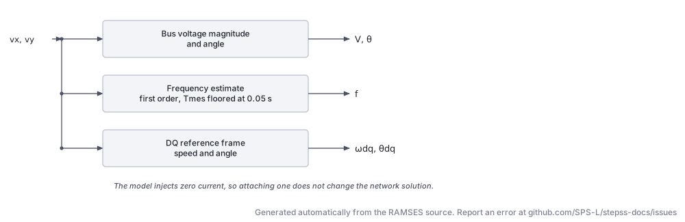
Description

A measurement-only injector: it injects zero current at its bus and exists purely to expose bus quantities as observables. It reports a filtered local frequency estimate computed the same way as the f_inj block, together with the bus voltage magnitude and angle and the speed and angle of the moving DQ reference frame. Attach one to any bus whose frequency you want to record without perturbing the solution.

The frequency estimate is a first-order filter on the bus voltage phasor. The measurement time constant is clamped to a floor of 0.05 s, so values below that have no effect.

Parameters

#	Name	Description	Unit
1	Tf	Frequency measurement time constant, recommended 0.05 to 0.10; values below 0.05 are clamped	s

Three additional parameters are set at initialisation: wnom (nominal angular frequency), vm0 and va0 (the initial bus voltage magnitude and angle).

Observables

Name	Description	Unit
f	Estimated bus frequency	pu of $f_{nom}$
vm	Bus voltage magnitude	pu
va	Bus voltage phase angle in the moving DQ frame, wrapping at $\pm\pi$	rad
thref	Accumulated angle of the DQ reference frame with respect to the nominally rotating frame, zero at $t = 0$	rad
dwref	Speed deviation of the DQ reference frame from nominal	rad/s

Caution

dwref and thref are only meaningful under $OMEGA_REF COI. With $OMEGA_REF SYN the reference frame rotates at nominal speed by construction, so both stay at zero.

Usage Example

INJEC  PMU  PMU_1041  1041  0.  0.  0.  0.  0.05 ;

All four participation and power fields are zero: the model neither consumes nor produces power.