Converter Models

Injector models for converter-interfaced units other than the WECC ones: a generic inverter-based generator, a photovoltaic unit, and grid-forming and grid-following converters. The WECC wind turbine and storage models are on WECC Wind and Storage.

The INJEC record these models are entered with, and the rules on model names, are on the Injector Models page.

IBG (inj_IBG): Inverter-Based Generator (Generic IBR)

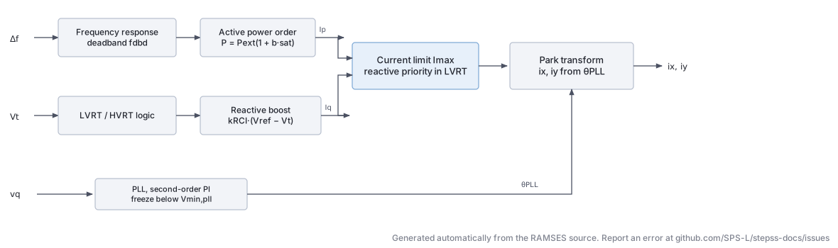
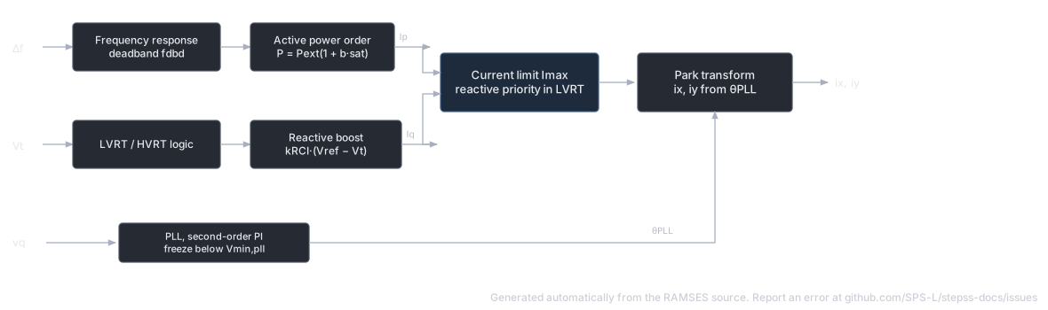
Description

A generic inverter-based generation model suitable for representing aggregated distributed generation or any grid-following IBR. The model includes a Phase-Locked Loop (PLL), inner current control with active ($I_p$) and reactive ($I_q$) current commands, LVRT/HVRT logic with voltage-dependent reactive current injection, frequency-responsive active power modulation, and reconnection logic after disconnection events.

Scientific Description

The PLL tracks the terminal voltage angle $\theta$ via a second-order PI controller with a freeze option below $V_{\mathrm{min,pll}}$:

$\frac{d\theta_{\mathrm{PLL}}}{dt} = \Delta\omega_{\mathrm{PLL}}, \qquad \frac{d\Delta\omega_{\mathrm{PLL}}}{dt} = k_{\mathrm{PLL}}\, v_q$

where $v_q$ is the $q$-axis terminal voltage in the PLL frame. The current commands $I_{p,\mathrm{cmd}}$ and $I_{q,\mathrm{cmd}}$ are derived from outer controls:

• Active power is modulated by frequency according to frequency deadband fdbd: $P = P_{\mathrm{ext}}\left(1 + b\,\mathrm{sat}(\Delta f - f_{\mathrm{start}}, f_{\mathrm{min}}, f_{\mathrm{max}})\right)$

• During voltage dips (LVRT), reactive current is boosted: $I_{q,\mathrm{boost}} = k_{\mathrm{RCI}}\,(V_{\mathrm{ref}} - V_t)$

• Current magnitude is limited to $I_{\mathrm{max}}$ with priority to reactive current during LVRT.

The injected currents in $x$-$y$ frame are:

$i_x = I_p \cos\theta_{\mathrm{PLL}} - I_q \sin\theta_{\mathrm{PLL}}$ $i_y = I_p \sin\theta_{\mathrm{PLL}} + I_q \cos\theta_{\mathrm{PLL}}$

Parameters

#	Name	Description	Unit
1	Imax	Maximum current magnitude	pu
2	IN	Nominal current	pu
3	Iprate	Active current ramp rate	pu/s
4	Tg	Generator time constant	s
5	Tm	Measurement filter time constant	s
6	tLVRT1	LVRT ride-through time threshold 1	s
7	tLVRT2	LVRT ride-through time threshold 2	s
8	tLVRTint	LVRT integration time	s
9	Vmax	Maximum voltage for operation	pu
10	tau	PLL response time	ms
11	Vminpll	Voltage below which PLL is frozen	pu
12	a	LVRT voltage-current curve slope
13	Vmin	Minimum LVRT voltage	pu
14	Vint	Intermediate LVRT voltage	pu
15	fmin	Minimum frequency for operation	pu
16	fmax	Maximum frequency for operation	pu
17	fstart	Frequency threshold for P modulation	pu
18	b	Frequency droop gain
19	fr	Reference frequency	pu
20	Tr	Reconnection delay after trip	s
21	Re	Grid equivalent resistance	pu
22	Xe	Grid equivalent reactance	pu
23	CM1	LVRT control mode flag
24	kRCI	Reactive current injection gain (LVRT)
25	kRCA	Reactive current absorption gain (HVRT)
26	m	Active-reactive current priority parameter
27	n	Active-reactive current priority parameter
28	dbmin	Frequency deadband lower limit	pu
29	dbmax	Frequency deadband upper limit	pu
30	HVRT	HVRT flag
31	LVRT	LVRT flag
32	CM2	Control mode 2 flag
33	Vtrip	Trip voltage threshold	pu

State Variables

Variable	Description
vxl, vyl	Filtered terminal voltage components
Vt	Terminal voltage magnitude
PLLPhaseAngle	PLL phase angle
Vm	Voltage magnitude measurement
Ip, Iq	Active and reactive current outputs
Ipcmd, Iqcmd	Current commands
Iqmax, Iqmin	Reactive current limits
Ipmax, Ipmin	Active current limits
DeltaW, DeltaWf	Frequency deviation and filtered value
Pgen, Qgen	Generated active and reactive power

Usage Example

Show the data record

INJEC  IBG  IBG1  BUS_GEN
      # FP FQ P Q: share of the power-flow injection (FP, FQ) or initial power (P in MW, Q in Mvar)
      1.  0.  0.  0.
      # Imax: Maximum current magnitude (pu)
      1.1
      # IN: Nominal current (pu)
      1.0
      # Iprate: Maximum rate of rise of the active current, in multiples of IN (pu/s)
      0.5
      # Tg: Generator time constant (s)
      0.02
      # Tm: Measurement filter time constant (s)
      0.01
      # tLVRT1: LVRT trip delay for Vmin <= Vm < Vint (s)
      0.15
      # tLVRT2: LVRT trip delay at Vm = a, upper end of the linear ramp (s)
      1.5
      # tLVRTint: LVRT trip delay at Vm = Vint, lower end of the linear ramp (s)
      0.3
      # Vmax: Maximum voltage for operation (pu)
      1.2
      # tau: PLL response time (ms)
      20.0
      # Vminpll: Voltage below which PLL is frozen (pu)
      0.1
      # a: Voltage below which the LVRT timer runs; upper end of the LVRT curve (pu)
      0.9
      # Vmin: Minimum LVRT voltage (pu)
      0.1
      # Vint: Intermediate LVRT voltage (pu)
      0.3
      # fmin: Underfrequency trip threshold on the filtered frequency, 50 Hz system (Hz)
      47.5
      # fmax: Overfrequency trip threshold on the filtered frequency, 50 Hz system (Hz)
      51.5
      # fstart: Frequency above which active power is reduced (Hz)
      50.2
      # b: Overfrequency power reduction gain: fraction of initial P per pu frequency above fstart (pu/pu)
      20.0
      # fr: While the frequency stays at or above fr the power reduction is held at its maximum (Hz)
      50.05
      # Tr: Reconnection delay after trip (s)
      1.0
      # Re: Resistance between the terminal bus and the controlled converter-side voltage (pu)
      0.0
      # Xe: Reactance between the terminal bus and the controlled converter-side voltage (pu)
      0.05
      # CM1: 1 enables the m and kRCI injection below dbmin with reactive current limit IN; 0 disables
      1
      # kRCI: Reactive current injection gain below dbmin, in IN per pu voltage (pu/pu)
      2.0
      # kRCA: Reactive current absorption gain above dbmax, in IN per pu voltage (pu/pu)
      1.5
      # m: Step of reactive current injected below dbmin, in multiples of IN; needs CM1 or CM2 = 1 (pu)
      0.0
      # n: Step of reactive current absorbed above dbmax, in multiples of IN (pu)
      0.0
      # dbmin: Lower edge of the voltage dead-band; reactive injection and Q priority below it (pu)
      0.9
      # dbmax: Upper edge of the voltage dead-band; reactive absorption above it (pu)
      1.1
      # HVRT: 1 enables the kRCA absorption term above dbmax; 0 disables it
      1
      # LVRT: 1 uses Vmin and Vint as the LVRT curve breakpoints; 0 replaces both with Vtrip
      1
      # CM2: 1 enables the m and kRCI injection below dbmin with reactive current limit 0.707 Imax; 0 disables
      0
      # Vtrip: Undervoltage trip threshold, used only when LVRT = 0 (pu)
      0.85
;

---

PV (inj_PV): Photovoltaic Generator

The data-file model name is PV (or inj_PV).

Note

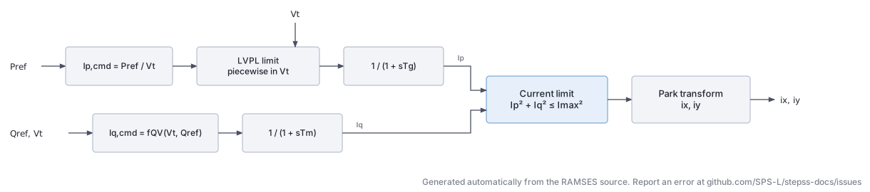
Callable since 3.79. Earlier releases compiled this model under no name, so a data file referring to it was rejected.

Description

A photovoltaic generator model with similar WECC-derived structure to the wind turbine models. The model includes a plant controller (voltage/reactive power regulation), an electrical controller (current limits, LVRT), and generator/converter representation. Unlike wind turbines, there is no mechanical drive train; the active power set-point follows an irradiance input or a fixed reference. LVRT/HVRT logic and current limiting are identical to the Type 4 wind model.

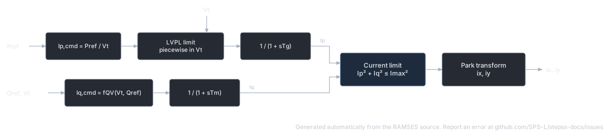
Scientific Description

The PV generator delivers active and reactive power through current commands:

$I_p = \frac{P_{\mathrm{ref}}}{V_t}, \qquad I_q = f_{\mathrm{QV}}(V_t, Q_{\mathrm{ref}})$

subject to the constraint $\sqrt{I_p^2 + I_q^2} \leq I_{\mathrm{max}}$. The inner current loop is a first-order filter:

$T_g \frac{dI_p}{dt} = I_{p,\mathrm{cmd}} - I_p, \qquad T_m \frac{dI_q}{dt} = I_{q,\mathrm{cmd}} - I_q$

Low-voltage power-logic (LVPL) limits active current during deep voltage sags via a piecewise-linear function of $V_t$ with breakpoints lvpnt0, lvpnt1, Lvpl1. HVRT and LVRT timers control disconnection and reconnection.

Parameters (selected)

#	Name	Description	Unit
1	Imax	Maximum converter current	pu
2	IN	Nominal current	pu
3	ratemax	Reconnection ramp rate	pu/s
4	Tg	Active current filter time constant	s
5	Tm	Reactive current filter time constant	s
6–9	LVRT timers	tLVRT1, tLVRT2, tLVRTint, Vmax	s, pu
10	kpll	PLL gain
11	Vminpll	PLL freeze voltage	pu
12–14	LVRT curve	a, Vmin, Vint
21–22	Re, Xe	Grid equivalent impedance	pu
23–29	Current control	CM1, kRCI, kRCA, m, n, dbmin, dbmax
34	BM	Battery module flag

Usage Example

Show the data record

INJEC  PV  PV1  BUS_PV
      # FP FQ P Q: share of the power-flow injection (FP, FQ) or initial power (P in MW, Q in Mvar)
      1.  1.  0.  0.
      # Imax: Maximum converter current; total current limit while Vm < 0.9 pu, and lower reactive current limit in normal operation (pu)
      1.1
      # IN: Nominal current; active and reactive current limit when Vm >= 0.9 pu, reactive absorption limit during a dip, and base of m and n (pu)
      1.0
      # ratemax: Maximum rate of rise of the active current Ip (decrease is not rate limited) (pu/s)
      0.5
      # Tg: Time constant of the active and reactive current lags (Ip and Iq) (s)
      0.02
      # Tm: Voltage measurement time constant (Vm and the voltage components used by the PLL) (s)
      0.01
      # tLVRT1: LVRT trip delay for Vmin <= Vm < Vint (s)
      0.15
      # tLVRT2: LVRT trip delay at Vm = a (upper end of the linear ramp) (s)
      1.5
      # tLVRTint: LVRT trip delay at Vm = Vint (lower end of the linear ramp up to tLVRT2 at Vm = a) (s)
      0.3
      # Vmax: Overvoltage threshold on the unfiltered voltage behind Re + jXe; reaching it trips the unit permanently (pu)
      1.2
      # kpll: PLL proportional gain from q-axis voltage to angle rate (integral gain fixed at zero) (rad/s/pu)
      20.0
      # Vminpll: Voltage below which the PLL angle is frozen (pu)
      0.1
      # a: Voltage below which the LVRT timer runs; upper end of the LVRT curve (pu)
      0.9
      # Vmin: LVRT curve: below this voltage the unit trips at once (used when LVRT = 1) (pu)
      0.1
      # Vint: LVRT curve intermediate voltage between the tLVRT1 plateau and the ramp (used when LVRT = 1) (pu)
      0.3
      # fmin: Underfrequency threshold on the filtered frequency; below it the unit trips permanently (Hz)
      47.5
      # fmax: Overfrequency threshold on the filtered frequency; above it the unit trips permanently (Hz)
      51.5
      # fstart: Frequency above which active power is reduced (Hz)
      50.2
      # b: Overfrequency active power reduction gain: fraction of initial P per pu frequency above fstart (50 Hz base) (pu/pu)
      20.0
      # fr: While filtered frequency >= fr the power reduction is held at its maximum; below fr it follows frequency again (Hz)
      50.05
      # Tr: Time the current output stays at zero after an LVRT trip before it is restored (at most 5 s takes effect) (s)
      1.0
      # Re: Resistance between the terminal bus and the controlled (converter side) voltage (pu)
      0.0
      # Xe: Reactance between the terminal bus and the controlled (converter side) voltage (pu)
      0.05
      # CM1: Reactive current injection mode 1: 1 enables the m and kRCI injection below dbmin, dip Iq limit Imax; 0 disables
      1
      # kRCI: Reactive current injection gain per pu voltage below dbmin (active if CM1, CM2 or CM3 is 1) (pu/pu)
      2.0
      # kRCA: Reactive current absorption gain per pu voltage above dbmax (active only if HVRT = 1) (pu/pu)
      1.5
      # m: Step reactive current injected below dbmin, as a multiple of IN (active if CM1, CM2 or CM3 is 1) (pu)
      0.0
      # n: Step reactive current absorbed above dbmax, as a multiple of IN (always active, independent of HVRT) (pu)
      0.0
      # dbmin: Lower edge of the voltage deadband on Vm; reactive injection below it (pu)
      0.9
      # dbmax: Upper edge of the voltage deadband on Vm; reactive absorption above it (pu)
      1.1
      # HVRT: 1 enables the kRCA absorption term above dbmax; 0 disables it (does not affect the Vmax trip)
      1
      # LVRT: 1 uses Vmin and Vint as LVRT curve breakpoints; 0 replaces both with 0.8 pu
      1
      # CM2: Reactive current injection mode 2: 1 enables m and kRCI injection and caps dip Iq at 0.707 Imax; 0 disables
      0
      # CM3: Reactive current injection mode 3: 1 enables m and kRCI injection, dip Iq limit sqrt(Imax^2 - Ipcmd^2) and a PI voltage term; 0 disables
      0
      # BM: Blocking mode: 1 zeroes the active current and drops the initial reactive current while Vm < 0.9 pu; 0 keeps both
      0
;

---

GFOR (inj_GFOR): Grid-Forming Converter (VSM)

The data-file model name is GFOR (or inj_GFOR).

Description

A grid-forming voltage source converter implementing Virtual Synchronous Machine (VSM) dynamics, modelled under the phasor approximation. The converter is an MMC-type VSC connected to the grid through its transformer (no LC filter); the DC side is not modelled (the DC voltage is assumed constant) so the focus is on the AC grid dynamics.

The modulated voltage magnitude is held at its setpoint $V_m^0$ in normal operation, while the phase angle $\delta_m$ is driven by a synthetic swing equation with inertia emulation ($H$) and oscillation damping ($D$) against a PLL estimate of the grid frequency. Participation in primary frequency control is optional, through the droop $R_{\mathrm{droop}}$. Overcurrents are limited by proportionally scaling the $d$-$q$ current vector back to the $I_{\mathrm{max}}$ circle with a small time constant.

Scientific Description

Reference frame. The $d$ axis is attached to the internal phase angle $\delta_m$ of the modulated voltage. Voltages and currents at the point of common coupling are transformed as:

$v_d = v_x\cos\delta_m + v_y\sin\delta_m, \qquad v_q = -v_x\sin\delta_m + v_y\cos\delta_m$

with the analogous transformation for the converter-side currents $i_{xt} = k\, i_x$, $i_{yt} = k\, i_y$, where $k = r\, S_{\mathrm{base}}/S_{\mathrm{nom}}$ converts to per-unit on the converter base.

Transformer. The voltage-current relationship across the connection transformer (resistance $R$, inductance $L$, ideal ratio $r$) in the $d$-$q$ frame is:

$v_{md} = \frac{v_d}{r} + R\, i_d - \omega_m L\, i_q, \qquad v_{mq} = \frac{v_q}{r} + R\, i_q + \omega_m L\, i_d$

PLL. The PLL only serves to estimate the grid angular frequency $\tilde{\omega}_g$ for the damping term. It is the same model as in the grid-following converter (see the PLL diagram there), with PI gains derived from the time constant $T_{\mathrm{pll}}$:

$K_{p\omega} = \frac{10}{\omega_N T_{\mathrm{pll}}}, \qquad K_{i\omega} = \frac{25}{\omega_N T_{\mathrm{pll}}^2}, \qquad \omega_N = 2\pi f_N$

The PLL is frozen (hysteresis) when the PCC voltage falls below 0.4 pu and reactivated when it recovers above 0.5 pu (fixed thresholds in this model).

Active power and phase angle control (VSM).

$2H\frac{d\omega_m}{dt} = P^* - P_{\mathrm{virt}} - D\left(\omega_m - \tilde{\omega}_g\right) + \frac{1 - \omega_m}{R_{\mathrm{droop}}}$

$\frac{d\delta_m}{dt} = \omega_N\left(\omega_m - \omega_{\mathrm{ref}}\right)$

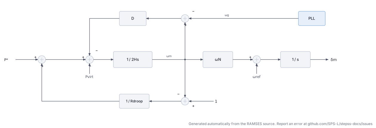
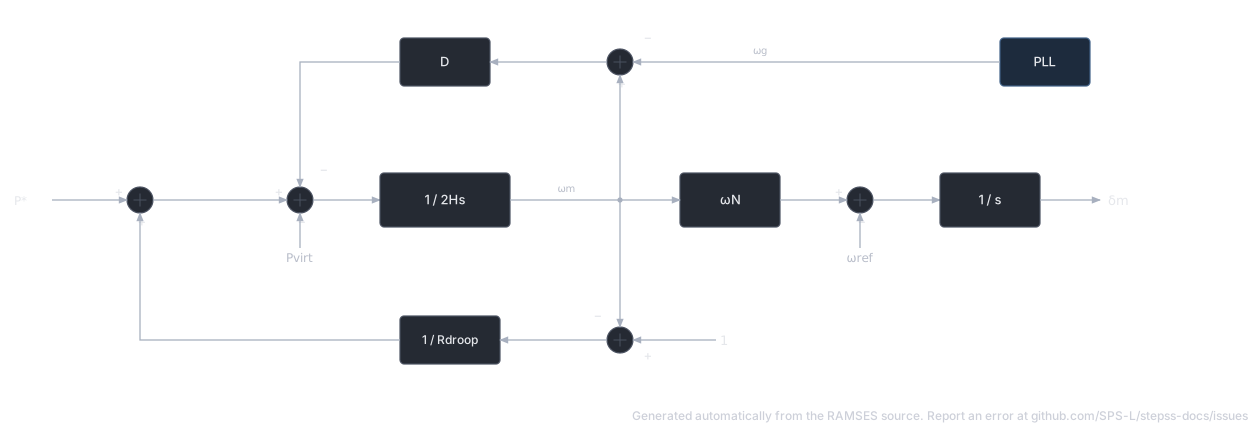
where $P^*$ is the active power setpoint and $P_{\mathrm{virt}}$ is the virtual power computed from the unsaturated currents:

$P_{\mathrm{virt}} = \frac{v_d}{r}\, i_d^* + \frac{v_q}{r}\, i_q^*$

$P_{\mathrm{virt}}$ equals the actual active power $P$ when the current is not limited, and yields improved large-disturbance stability while the current is limited (the angle dynamics do not wind up).

Current limitation. The currents $(i_d^*, i_q^*)$ that would result from normal voltage control (i.e. $v_{md} = V_m^0$, $v_{mq} = 0$) are first determined from:

$V_m^0 = \frac{v_d}{r} + R\, i_d^* - \omega_m L\, i_q^*, \qquad 0 = \frac{v_q}{r} + R\, i_q^* + \omega_m L\, i_d^*$

The current overload ratio $\rho = \sqrt{(i_d^*)^2 + (i_q^*)^2}\,/\,I_{\mathrm{max}}$ is passed through a first-order lag with time constant $T_e$ (typically 1 ms) and a non-windup lower limit of 1, giving $\rho_s$. Both current components are then decreased in the same proportion:

$i_{ds}^* = \frac{i_d^*}{\rho_s}, \qquad i_{qs}^* = \frac{i_q^*}{\rho_s}$

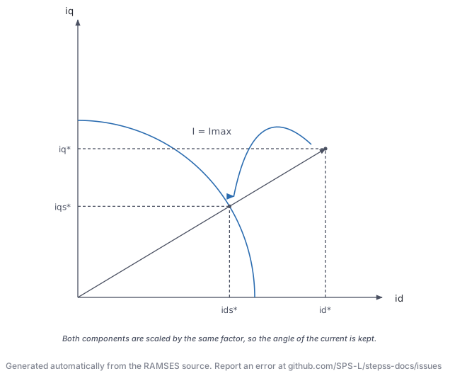
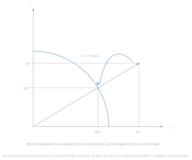
and the modulated voltage is set to the value that yields the saturated currents:

$v_{md} = \frac{v_d}{r} + R\, i_{ds}^* - \omega_m L\, i_{qs}^*, \qquad v_{mq} = \frac{v_q}{r} + R\, i_{qs}^* + \omega_m L\, i_{ds}^*$

When $I < I_{\mathrm{max}}$: $\rho_s = 1$, the currents are unsaturated, and $v_{md} = V_m^0$, $v_{mq} = 0$.

Parameters

Default values correspond to a 1100 MVA converter. Per-unit values refer to the nominal apparent power of the converter.

#	Name	Description	Unit	Default
1	R	Resistance of connection transformer	pu	0.005
2	L	Inductance of connection transformer	pu	0.15
3	r	Ratio of ideal transformer		1.02
4	Snom	Nominal apparent power	MVA	1100
5	H	Inertia constant	s	5.0
6	D	Damping constant of virtual synchronous machine		300
7	Tpll	Time constant of PLL	s	0.1
8	Rdroop	Droop of primary frequency control	pu	999
9	Imax	Maximum current (typically 1–1.2)	pu	1.0
10	Te	Time constant of current saturation	s	0.001

A very large Rdroop (e.g. 999) effectively disables participation in primary frequency control.

Five additional parameters are computed at initialization from the power-flow solution: k (current conversion factor), vmx0, vmy0 (components of the initial modulated voltage), Vmo (its magnitude $V_m^0$, i.e. the voltage setpoint) and Po (the active power setpoint $P^*$, pu on Snom base). Vmo and Po can be modified during the simulation with CHGPRM disturbances to change the voltage and active power setpoints.

State Variables

The model has 33 states (2 output currents + 31 internal). Key internal states:

Variable	Description	Unit
wref	Angular speed of reference axes	pu
ixt, iyt	Converter-side currents (on Snom base)	pu
Vm, deltam	Modulated voltage magnitude and phase angle	pu, rad
V	Voltage magnitude at PCC	pu
mult_pll	PLL freezing factor (hysteresis output)
w_pll, theta_pll	PLL frequency and angle estimates	pu, rad
P, Pvirt	Active power and virtual power (on Snom base)	pu
omegam	Angular frequency of modulated voltage	pu
vd, vq, id, iq	PCC voltage and current in $d$-$q$ frame	pu
id*, iq*	Unsaturated currents	pu
id*s, iq*s	Saturated currents	pu
rho, rhos	Current overload ratio and its saturated value
Q	Reactive power (on Snom base)	pu

Observables: P, Pvirt, Q, Vm, vmd, vmq, deltam, omegam, w_pll, I, id, id*, id*s, iq, iq*, iq*s, rho, rhos.

Usage Example

A 1100 MVA grid-forming converter:

Show the data record

INJEC  GFOR  HVDC  A
      # FP FQ P Q: share of the power-flow injection (FP, FQ) or initial power (P in MW, Q in Mvar)
      1.  1.  0.  0.
      # R: Resistance of connection transformer (pu)
      0.005
      # L: Inductance of connection transformer (pu)
      0.15
      # r: Ratio of the ideal connection transformer (pu/pu)
      1.02
      # Snom: Nominal apparent power (MVA)
      1100.
      # H: Inertia constant (s)
      5.0
      # D: Damping constant of virtual synchronous machine
      300.
      # Tpll: Time constant of PLL (s)
      0.100
      # Rdroop: Droop of primary frequency control (pu)
      999.
      # Imax: Maximum current (typically 1–1.2) (pu)
      1.0
      # Te: Time constant of current saturation (s)
      0.001
;

Note

At operating points where the initial current is below $I_{\mathrm{max}}$, RAMSES reports a small initial mismatch on the $\rho_s$ lag equation (“INJECTORS NOT IN STEADY STATE”). This is benign: $\rho_s$ starts exactly at its lower limit of 1 and is clamped there by the discrete update within the first time step.

---

GFOL (inj_GFOL): Grid-Following Converter

The data-file model name is GFOL (or inj_GFOL).

Description

A grid-following voltage source converter modelled under the phasor approximation. As for the grid-forming model, the converter is an MMC-type VSC connected through its transformer (no LC filter) and the DC side is not modelled. The model is rather detailed: it includes measurement low-pass filters, a PLL with blocking/unblocking hysteresis, outer active power and voltage/reactive power control loops, inner $d$-$q$ current control loops, a rate-limited $d$-axis current limit with priority to the reactive current, and a piecewise-linear dynamic voltage support characteristic.

Scientific Description

Reference frame. The VSC control frame $(d, q)$ tracks the PCC voltage phasor through the PLL angle $\tilde{\delta}_g$ (state theta_pll):

$v_d = v_x\cos\tilde{\delta}_g + v_y\sin\tilde{\delta}_g, \qquad v_q = -v_x\sin\tilde{\delta}_g + v_y\cos\tilde{\delta}_g$

with the analogous transformation for the converter-side currents ($i_{xt} = k\, i_x$, $k = r\, S_{\mathrm{base}}/S_{\mathrm{nom}}$). In steady state $v_q = 0$ and $v_d = V$.

Phase Locked Loop.

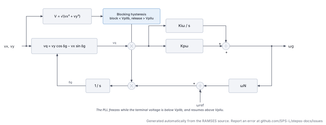
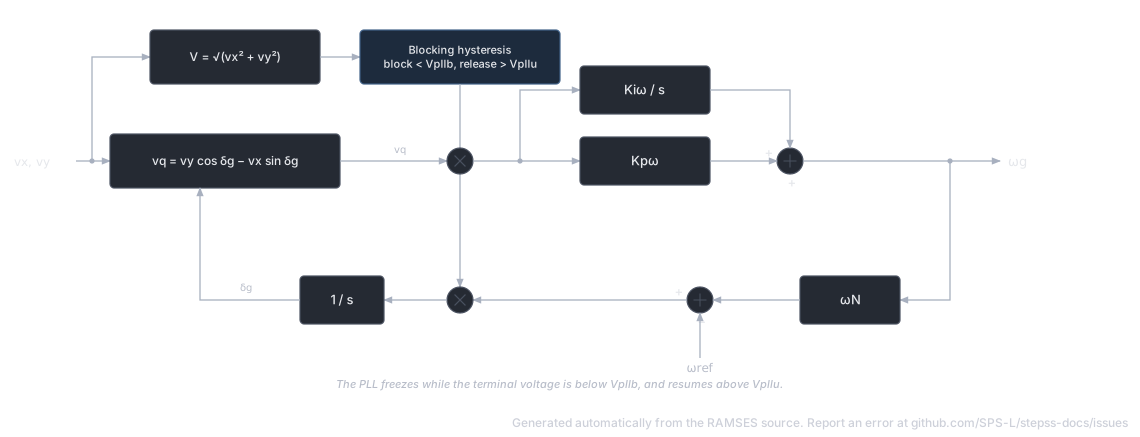
The $q$-axis voltage error drives a PI controller whose output is the grid frequency estimate $\tilde{\omega}_g$ (state w_pll); integrating $\omega_N(\tilde{\omega}_g - \omega_{\mathrm{ref}})$ gives the PLL angle. The PI gains follow from the PLL response time $\tau$:

$K_{p\omega} = \frac{10}{\omega_N \tau}, \qquad K_{i\omega} = \frac{25}{\omega_N \tau^2}, \qquad \omega_N = 2\pi f_N$

The PLL is blocked once the PCC voltage $V$ falls below Vpllb and reactivated once $V$ recovers above Vpllu (hysteresis).

Inner current control.

$v_{md} = \frac{v_d}{r} - \tilde{\omega}_g L\, i_q + \left(K_p + \frac{K_i}{s}\right)\left(i_d^{\mathrm{ref}} - i_d\right)$

$v_{mq} = \tilde{\omega}_g L\, i_d + \left(K_p + \frac{K_i}{s}\right)\left(i_q^{\mathrm{ref}} - i_q\right)$

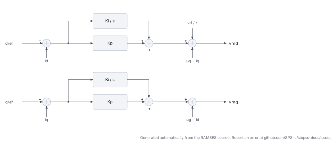
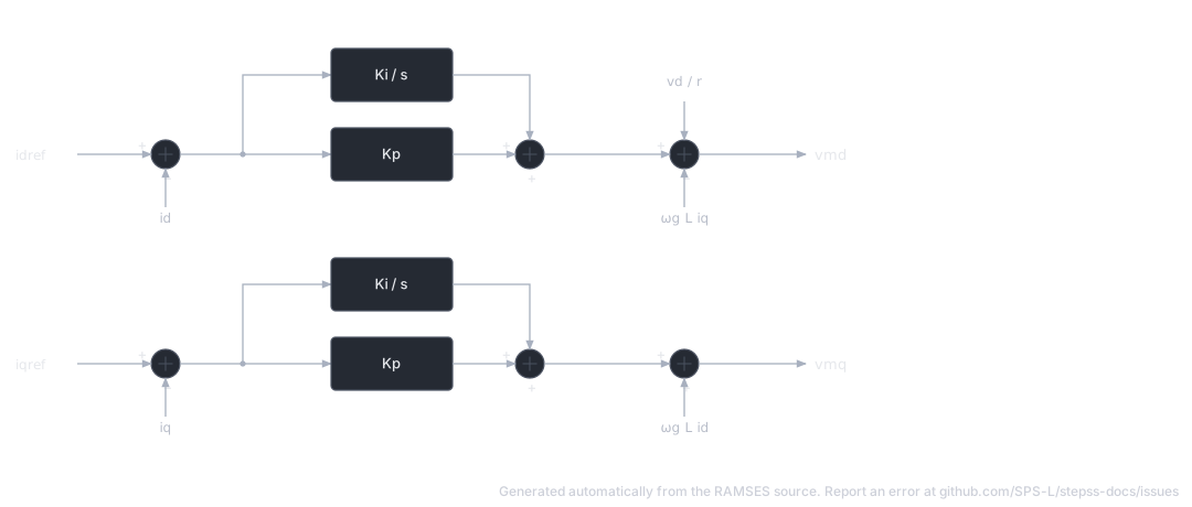
combined with the transformer voltage-current relationship in the $d$-$q$ frame:

$v_{md} = \frac{v_d}{r} + R\, i_d - \tilde{\omega}_g L\, i_q, \qquad v_{mq} = \frac{v_q}{r} + R\, i_q + \tilde{\omega}_g L\, i_d$

Active power control.

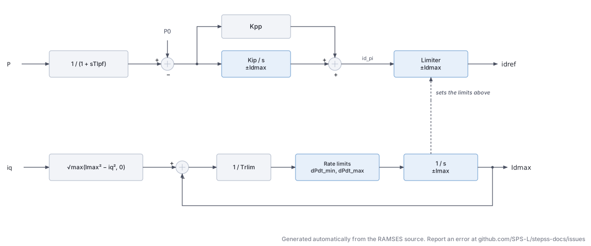
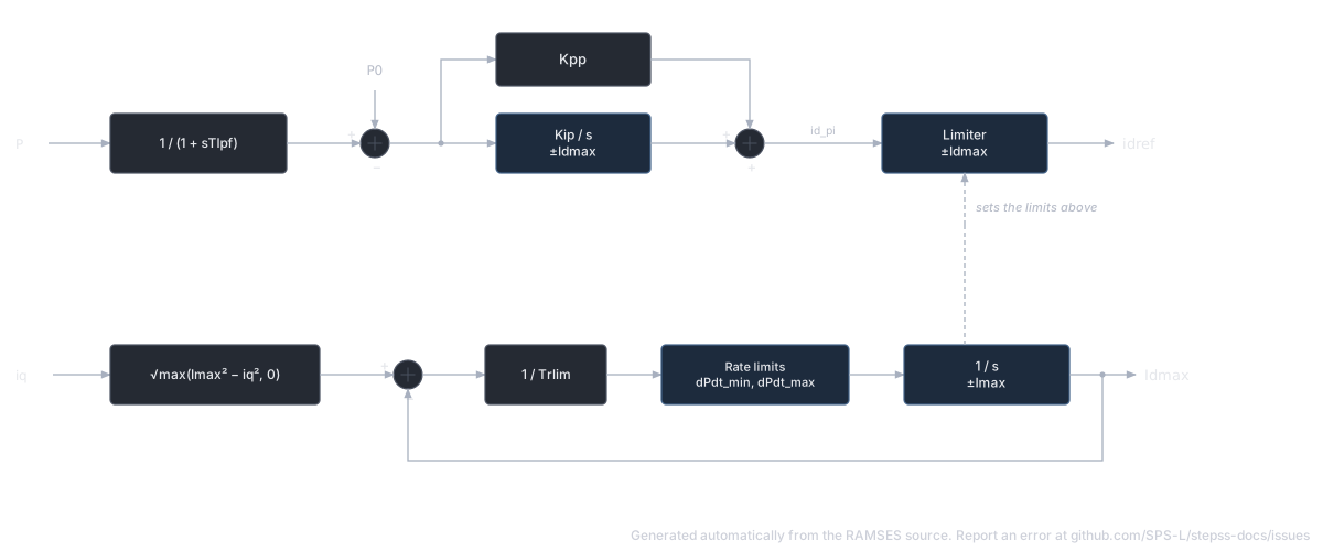
The measured active power is filtered with time constant $T_{\mathrm{lpf}}$ and compared with the setpoint $P^0$; a PI controller ($K_{pp}$, $K_{ip}$) with non-windup limits $\pm I_d^{\max}$ produces $i_d^{\mathrm{ref}}$. The limit gives priority to the reactive current:

$I_d^{\max,\mathrm{stat}} = \sqrt{\max\left(I_{\mathrm{max}}^2 - i_q^2,\; 0\right)}$

and $I_d^{\max}$ tracks this static value through a first-order lag ($T_{\mathrm{rlim}}$, typically 0.002 s) with rate limits dPdt_min/dPdt_max, limiting in particular the rate of recovery of the active current after it has been decreased by an increase of $i_q$.

Voltage / reactive power control.

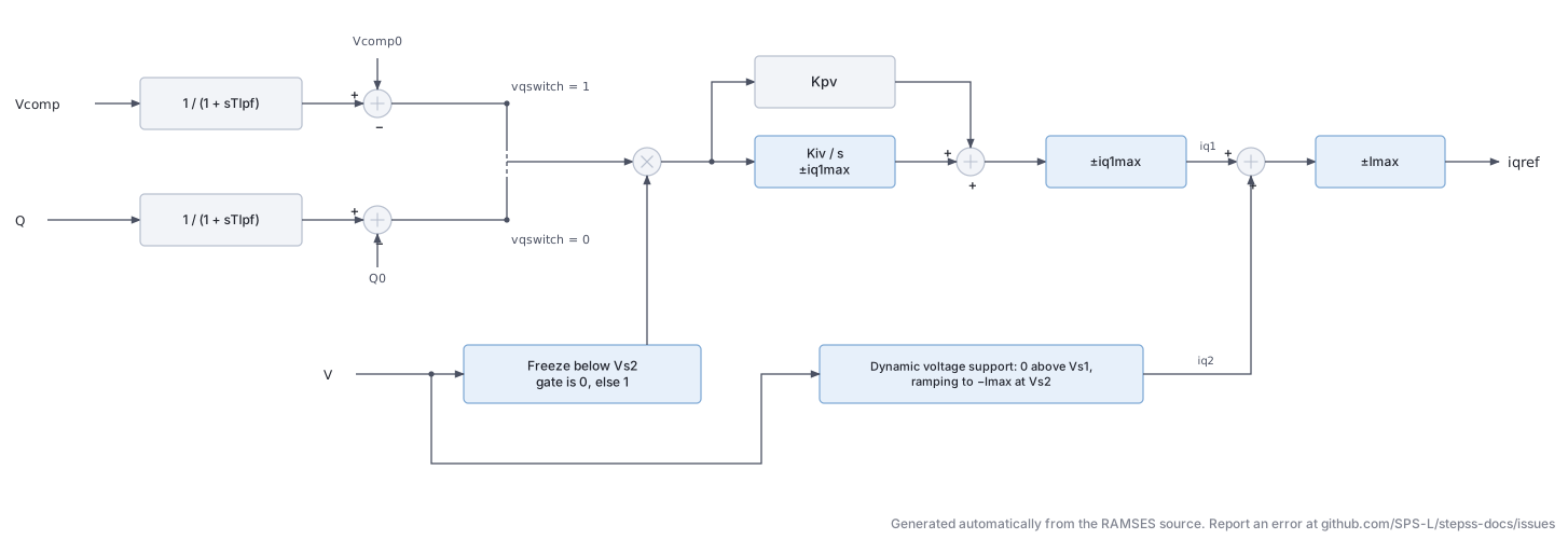
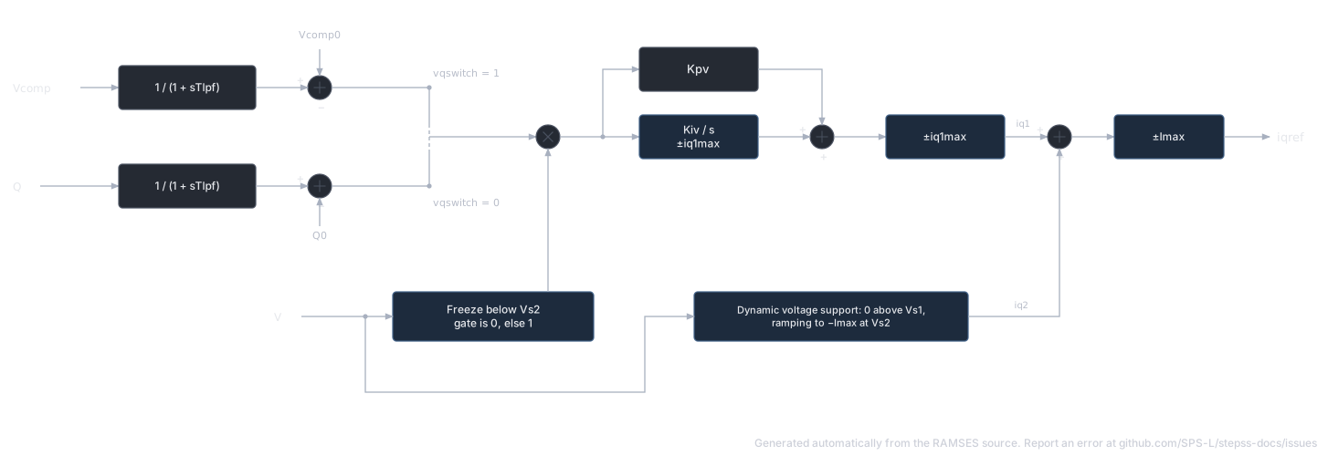
Depending on vqswitch, either the compensated voltage or the reactive power is controlled:

$V_c = \left|\frac{\bar{v}}{r} + (R_c + jX_c)\,\bar{i}\right| \quad (\texttt{vqswitch}=1), \qquad Q = \frac{v_q}{r} i_d - \frac{v_d}{r} i_q \quad (\texttt{vqswitch}=0)$

The controlled quantity is filtered ($T_{\mathrm{lpf}}$) and its deviation from setpoint drives a PI controller ($K_{pv}$, $K_{iv}$) with non-windup limits $\pm i_{q1}^{\max}$, giving the component $i_{q1}$. The error is zeroed (controller frozen) while $V < V_{s2}$. A second component $i_{q2}$ implements dynamic voltage support as a piecewise-linear function of $V$: zero above $V_{s1}$, decreasing linearly to $-I_{\mathrm{max}}$ at $V_{s2}$, constant below. The total $i_{q1} + i_{q2}$, limited to $\pm I_{\mathrm{max}}$, is the reactive current reference $i_q^{\mathrm{ref}}$.

With $R_c = R$, $X_c = \omega L$ and $r = 1$, controlling $V_c$ amounts to controlling the magnitude of the modulated voltage.

Parameters

Default values correspond to a 1200 MVA converter. Per-unit values refer to the nominal apparent power of the converter.

#	Name	Description	Unit	Default
1	R	Phase reactor resistance	pu	0.005
2	L	Phase reactor inductance	pu	0.15
3	r	Ratio of ideal transformer		1.02
4	Snom	Nominal apparent power	MVA	1200
5	Rc	Resistance used in compensated voltage	pu	0.005
6	Xc	Reactance used in compensated voltage	pu	0.15
7	Kp	Current control: proportional gain		0.573
8	Ki	Current control: integral gain		6.0
9	Tlpf	Measurement time constant (low-pass filter)	s	0.0033
10	Kpp	Active power control: proportional gain		0.0333
11	Kip	Active power control: integral gain		10.0
12	Trlim	Time constant of the $I_d^{\max}$ rate limiter	s	0.002
13	dPdt_min	Min rate of change of the $d$-current limit	pu/s	-999
14	dPdt_max	Max rate of change of the $d$-current limit	pu/s	10.0
15	Kpv	Reactive power control: proportional gain		0.1667
16	Kiv	Reactive power control: integral gain		50.0
17	tau	Response time of PLL	s	0.10
18	Vpllb	Voltage below which the PLL is blocked	pu	0.4
19	Vpllu	Voltage above which the PLL is unblocked	pu	0.5
20	Imax	Maximum current (typically 1–1.2)	pu	1.0
21	Vs1	Voltage below which dynamic reactive support starts	pu	-1000
22	Vs2	Voltage at which reactive support is maximum ($V_{s2} < V_{s1}$)	pu	-2000
23	iqmax	Limit (±) on quadrature current component $i_{q1}$	pu	1.001
24	vqswitch	1 = voltage control, 0 = reactive power control	flag	1

Setting Vs1 and Vs2 to large negative values (as in the defaults above) disables the dynamic voltage support; a more elaborate control is recommended for that function. Typical values of Kiv are 50 pu/s for voltage control and 10 pu/s for reactive power control.

Six additional parameters are computed at initialization from the power-flow solution: k (current conversion factor), P0, Q0 (active/reactive power setpoints, pu on Snom base), Vc0 (compensated voltage setpoint), Imin and iq1max ($= \min(\texttt{iqmax}, I_{\mathrm{max}})$). P0, Q0 and Vc0 can be modified during the simulation with CHGPRM disturbances.

State Variables

The model has 52 states (2 output currents + 50 internal). Key internal states:

Variable	Description	Unit
wref	Angular speed of reference axes	pu
ixt, iyt	Converter-side currents (on Snom base)	pu
mult_pll	PLL freezing factor (hysteresis output)
w_pll, theta_pll	PLL frequency and angle estimates	pu, rad
V, vd, vq	PCC voltage magnitude and $d$-$q$ components	pu
id, iq	Converter currents in $d$-$q$ frame	pu
vmd, vmq	Modulated voltage components	pu
Md, Mq	Current-control PI outputs	pu
Idmax_stat, Idmax, Idmin	Static / rate-limited / minimum $d$-current limits	pu
P, Pfil	Active power and its filtered value	pu
id_pi, idref	Active-power PI output and $d$-current reference	pu
Vc, Vcfil	Compensated voltage and its filtered value	pu
Q, Qfil	Reactive power and its filtered value	pu
mult_V	Voltage/reactive controller freezing factor
iq_1, iq_2, iqref	Reactive current components and reference	pu

Observables: P_MW, Q_Mvar, Vc, Vm, vmd, vmq, I, w_pll, theta_pll_deg, mult_pll, Idmax, Md, idref, id, id_pi, iq_1, iq_2, iqref, iq.

Usage Example

A 1200 MVA grid-following converter (record spanning multiple lines):

Show the data record

INJEC  GFOL  HVDC1  A
      # FP FQ P Q: share of the power-flow injection (FP, FQ) or initial power (P in MW, Q in Mvar)
      1.  1.  0.  0.
      # R: Phase reactor resistance (pu)
      0.005
      # L: Phase reactor inductance (pu)
      0.15
      # r: Ratio of the ideal connection transformer (pu/pu)
      1.02
      # Snom: Nominal apparent power (MVA)
      1200.
      # Rc: Resistance used in compensated voltage (pu)
      0.005
      # Xc: Reactance used in compensated voltage (pu)
      0.15
      # Kp: Current control: proportional gain
      0.5730
      # Ki: Current control: integral gain
      6.
      # Tlpf: Measurement time constant (low-pass filter) (s)
      0.0033
      # Kpp: Active power control: proportional gain
      0.0333
      # Kip: Active power control: integral gain
      10.
      # Trlim: Time constant of the I_d^max rate limiter (s)
      0.002
      # dPdt_min: Min rate of change of the d-current limit (pu/s)
      -999.
      # dPdt_max: Max rate of change of the d-current limit (pu/s)
      10.
      # Kpv: Reactive power control: proportional gain
      0.1667
      # Kiv: Reactive power control: integral gain
      50.
      # tau: Response time of PLL (s)
      0.10
      # Vpllb: Voltage below which the PLL is blocked (pu)
      0.4
      # Vpllu: Voltage above which the PLL is unblocked (pu)
      0.5
      # Imax: Maximum current (typically 1–1.2) (pu)
      1.000
      # Vs1: Voltage below which dynamic reactive support starts (pu)
      -1000
      # Vs2: Voltage below which reactive support is maximum and the V/Q PI is frozen (pu)
      -2000
      # iqmax: Limit (±) on quadrature current component i_q1 (pu)
      1.001
      # vqswitch: 1 = voltage control, 0 = reactive power control (flag)
      1
;