

Stabilizers and Limiters
The power system stabilizers and over-excitation limiters that the IEEE exciter variants are combined with. They are not entered on their own: each is part of a variant such as ST1A_PSS2B or AC1A_MAXEX2.
The EXC sub-record these models are entered with, and the table of IEEE model variants, are on the Exciter Models page.
PSS Models
Section titled “PSS Models”Power System Stabilizers (PSS) inject an additional signal at the AVR summation point to damp electromechanical oscillations. All variants listed in the IEEE model variants table include one of the PSS types described here.
PSS2B: Dual-Input Stabilizer
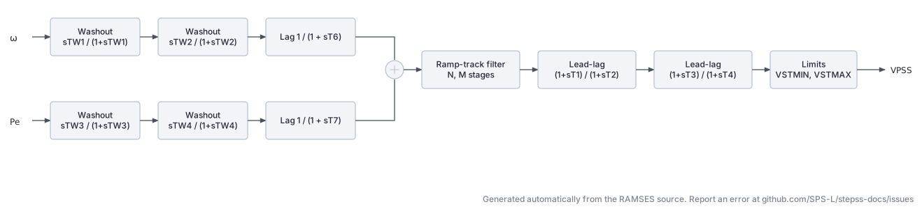
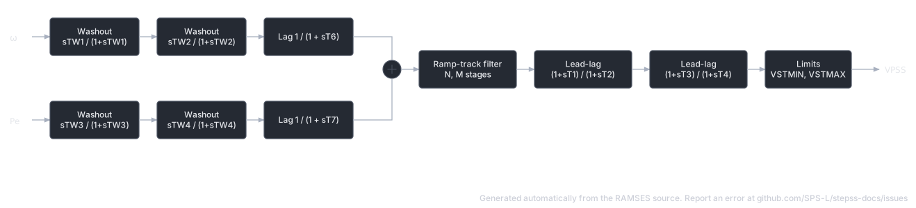
Section titled “PSS2B: Dual-Input Stabilizer”PSS2B accepts two input signals (typically speed and electrical power ) and processes them through independent washout chains before combining. It corresponds to IEEE Std 421.5-2016 Type PSS2B.
Channel 1 (input 1 washout):
Channel 2 (input 2 washout):
Combination and lead-lag chain (variant M=5, N=1 implemented):
PSS2B Parameters (additional to base exciter):
| Parameter | Description |
|---|---|
speedinput | Input selection (1=speed+power, 2=power+speed) |
TW1, TW2 | Channel 1 washout time constants |
T6 | Channel 1 filter |
TW3, TW4 | Channel 2 washout time constants |
T7, KS2 | Channel 2 filter gain and time constant |
KS3 | Channel coupling gain |
T8, T9 | Ramp-tracking filter |
KS1 | Overall PSS gain |
T1–T4, T10, T11 | Lead-lag time constants |
VS1MIN, VS1MAX | Input 1 limits |
VS2MIN, VS2MAX | Input 2 limits |
VSTMIN, VSTMAX | Output limits |
PSS3B: Two-Input Second-Order Filter Stabilizer
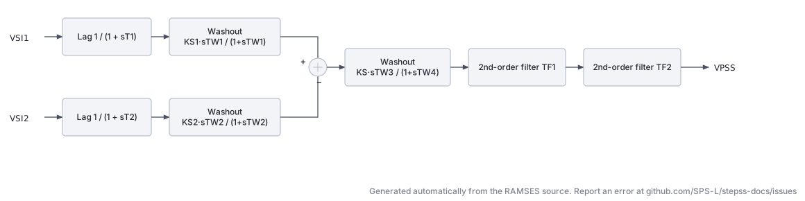
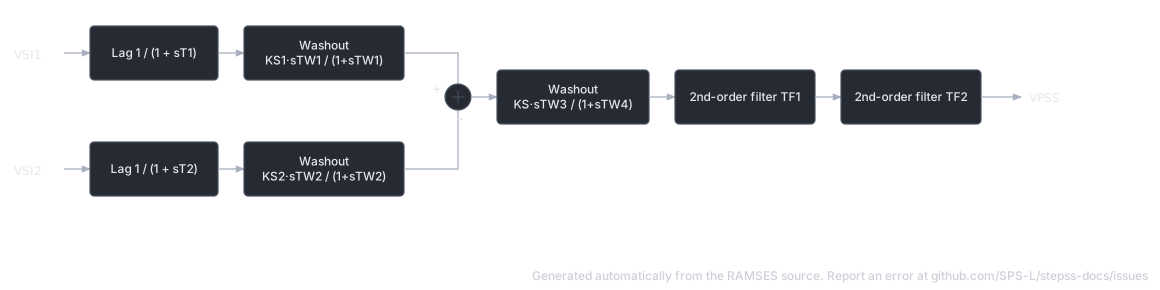
Section titled “PSS3B: Two-Input Second-Order Filter Stabilizer”PSS3B processes two input channels through measurement filters and washout stages, then combines them and applies two cascaded second-order lead-lag filters. It corresponds to IEEE Std 421.5-2016 Type PSS3B.
PSS3B Parameters (additional):
| Parameter | Description |
|---|---|
speedinput | Input mode selection |
T1, KS1, TW1 | Channel 1 filter, gain, washout |
T2, KS2, TW2 | Channel 2 filter, gain, washout |
KS, TW3, TW4 | Combined washout gain and time constants |
A1–A8 | Second-order filter coefficients |
VSTMIN, VSTMAX | Output limits |
PSS4B: Three-Band Multi-Input Stabilizer
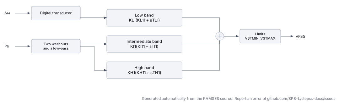
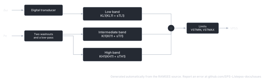
Section titled “PSS4B: Three-Band Multi-Input Stabilizer”PSS4B is a three-band stabilizer that separates the speed deviation signal into low-, intermediate-, and high-frequency components. Each band uses a pair of lead-lag filters. This model corresponds to IEEE Std 421.5-2016 Type PSS4B.
The speed signal passes through a digital transducer (tf2p2z) to obtain the low/intermediate input. Electrical power passes through two washouts and a low-pass filter to derive the high-frequency component .
Low-frequency band ( input):
Intermediate-frequency band (same input):
High-frequency band ( input):
PSS4B Parameters (additional):
| Parameter | Description |
|---|---|
H | Generator inertia constant (for high-freq path) |
KL1, KL11, TL1, TL2 | Low-band filter 1 |
KL2, KL17, TL7, TL8 | Low-band filter 2 |
KL, VLMax, VLMin | Low-band gain and limits |
KI1, KI11, TI1, TI2 | Intermediate-band filter 1 |
KI2, KI17, TI7, TI8 | Intermediate-band filter 2 |
KI, VIMax, VIMin | Intermediate-band gain and limits |
KH1, KH11, TH1, TH2 | High-band filter 1 |
KH2, KH17, TH7, TH8 | High-band filter 2 |
KH, VHMax, VHMin | High-band gain and limits |
VSTMax, VSTMin | Total output limits |
IEEEST: Single-Input Stabilizer
Section titled “IEEEST: Single-Input Stabilizer”The IEEEST is a general-purpose single-input PSS with selectable input signal (speed deviation, electrical power, or computed accelerating power). It corresponds to IEEE Std 421.5-2016 Type PSS1A. Two second-order lead-lag filters provide frequency shaping before two first-order lead-lags and a washout stage.
Input selection (speedinput): 1 = rotor speed deviation, 3 = electrical power, 4 = computed accelerating power ().
IEEEST Parameters (additional):
| Parameter | Description |
|---|---|
speedinput | Input mode (1, 3, or 4) |
A1–A6 | Second-order filter coefficients |
T1–T6 | Lead-lag and washout time constants |
KS | Overall PSS gain |
LSMIN, LSMAX | Output limits |
KS4 | Inertia constant for accelerating power (= 2H) |
TW4 | Derivative filter time constant |


STAB3: Power-Input Stabilizer
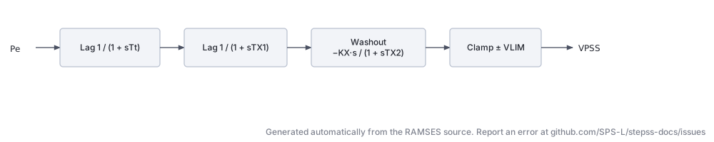
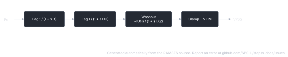
Section titled “STAB3: Power-Input Stabilizer”The STAB3 is a simplified PSS that takes electrical power as input, applies two sequential first-order filters and a washout-type derivative block, producing a stabilizing signal.
STAB3 Parameters:
| Parameter | Description |
|---|---|
Tt | Input measurement time constant |
TX1 | First filter time constant |
KX | Stabilizer gain |
TX2 | Washout time constant |
VLIM | Output limit |
OEL and Limiter Models
Section titled “OEL and Limiter Models”Over-Excitation Limiters (OEL) prevent sustained field current overloads that would thermally damage the field winding. They generate a signal that reduces the AVR output when field current exceeds thermal limits.
MAXEX2: Field Current Limiter with Timer and Hysteresis
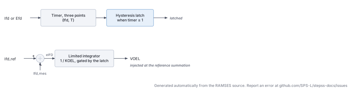
Section titled “MAXEX2: Field Current Limiter with Timer and Hysteresis”The MAXEX2 is a field current limiter derived from IEEE work, using a simplified three-point piece-wise linear timer It is designed for the EXST1/ST1A topology where the OEL output is injected at the reference summation point (not the LV gate).
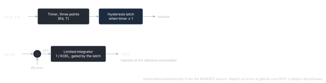
Timer phase: The measured current (selected as either field current or via parameter IC) drives a timer3 block with three operating points. The hyst block latches when timer ≥ 1.
Integral phase: Once latched, the error drives a limited integrator:
is subtracted from the reference (, i.e. Negative reduces reference).
MAXEX2 Parameters:
| Parameter | Description |
|---|---|
IC | Input selection: 0 = , 1 = |
IFDrated | Rated field current (reference) |
IFD1, TIME1 | Timer point 1 (current level, allowable duration) |
IFD2, TIME2 | Timer point 2 |
IFD3, TIME3 | Timer point 3 |
IFDDES | Desired steady-state field current after limiting |
KMX | Integrator time constant inverse (1/KMX = integration rate) |
VLOW | Lower limit of OEL output (e.g. −1.0 pu) |
Integral OEL (_lim variants)
Section titled “Integral OEL (_lim variants)”The simple integral OEL used in AC8B_lim, ST1A_lim, SEXS_STAB3_lim, and ENTSOE_lim variants computes the over-excitation signal through a clamped integrator acting on the difference between measured field current and , with an input clamp at .
A stator current limiter (SCL) with analogous structure acts on relative to .
Integral OEL Parameters (in _lim variants):
| Parameter | Description |
|---|---|
IFDN | Nominal field current (OEL trigger at 1.05×) |
TOEL | OEL integrator time constant |
LOEL | OEL integrator lower limit |
UOEL | OEL integrator upper limit |
KOEL | OEL output gain |
OELLI | OEL output lower limit |
IGN | Nominal stator current (SCL trigger at 1.025×) |
TSCL | SCL integrator time constant |
LSCL | SCL integrator lower limit |
USCL | SCL integrator upper limit |
KSCL | SCL output gain |
SCLLI | SCL output lower limit |
For full documentation of the CODEGEN DSL primitives used in these models (tf1p, tf1p1z, tf1plim, inlim, pictl, etc.), see the CODEGEN Blocks reference.

